LERC is a kick-ass approach to 2D raster data compression, supported in GDAL since version 3.3. You can use it for lossless compression but it is also able to throw away some bits of information for smaller data sizes. You tell it which level of Z error is acceptable for your values and it will use that freedom to change the values of neighboring cells to do its magic. Z means the “data” axis here, of a single-band in a 2D raster, X and Y are the coordinates, or rather the locations of the data values in the raster, which are obviously not changed.
I thought it would be nice to show what it actually results in, you can read up on the details elsewhere if you want. Look at the images in full resolution please.
I used a global SRTM DEM with a Z value in full meters (no floating point values but integers) and applied LERC on it in three ways: Lossless, with a maximum Z error of 1 meter and a maximum Z error of 10 meters. Zstandard compression was always used.
The original GeoTIFF file was already very well compressed with Zstandard level 15 and a horizontal predictor; at ~1296000 x ~417600 pixels it has a size of 86 gigabytes including overviews.
- Original (ZSTD level 15): 86 GB
- LERC_ZSTD (lossless): 105G
- LERC_ZSTD (maximum Z error of 1): 81G
- LERC_ZSTD (maximum Z error of 10): 21G
Cool, so if we don’t care about an error of 10 meters, we can have a global DEM (well, as global as SRTM is with its 60° cut-off) at ~30 meters pixel resolution in 21 gigabytes. But what does that actually look like then and how will this error appear? Well, check it out:
Here are some samples visualised with a greyscale color ramp (locally adjusted, so the lowest value in the image is black, the highest value is white). They are shown at a 1:1 resolution, one pixel in the image (if you look at it at 100%) is one cell of the DEM data. The left image is lossless, the middle one was allowed an Z error of 1 meter, the right one 10 meters.
Mountainous, here the values range from 0 meters to about 2000 meters:


You can hardly see a difference, at least visually.
“Mediumish”, values between ~100 and ~500 meters:


At the 10 meter error level you can see a significant terracing effect.
Plains, values all around 100 meters:


You can see some structures collapsing into flat areas in the 1 meter version and oh wow that 10 meters version looks like upscaled pixels.
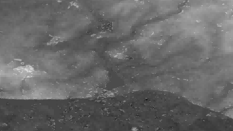
Time to zoom in! I picked a less flat area again because it makes it easier to understand. Here the values are between ~100 and ~300 meters:

So what do we see here? Neighboring cells with the same values compress better so LERC is shifting the values around (within the allowed error), creating terraces of same-valued cells. If you look closely you can see that there is also a visible pattern of squarish structures. Those are the blocks or windows in which LERC looks at the data and does its adjustments, in this case they were 8×8 pixels wide. Note: What LERC does exactly is a bit more complex than “try to make neighboring values the same”, it actually looks at the bits required to store the values within a block and optimized that within the error tolerance.
And now you know what LERC can do, if you give it a error level to play with.
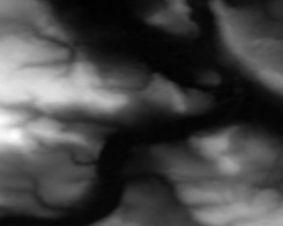
For reference, here is that same-ish area with the error tolerance at 1 meter:

You have to zoom in quite a bit more to be able to see the effects here due to the nature of the data in this extent in combination with the particular error tolerance:


The larger the zonal differences of your Z values are to each other and in relation to the error tolerance, the less distinguished will this effect be. If there are steps of 100 meters between neighboring pixels, an extra error of 10 meters won’t do much of a difference. But in more flat areas it will have significant “terracing” effects as you could see above. This is similar to “banding” effects in images where there is little variation in color, e. g. a blue sky or an artificial color gradient, and you look at it in a setup that has a color bit depth on a resolution your human eyes can distinguish.
So if you want to use LERC with a lossy approach, think hard about what is going to happen with your data later. What kind of analysis will be performed, how will it be “looked” at, what will be calculated. Do it smart and you can have a predictable/controllable lossy compression with seriously small file sizes, do it without thinking and your data will lead to misinterpretation and apocalypse.