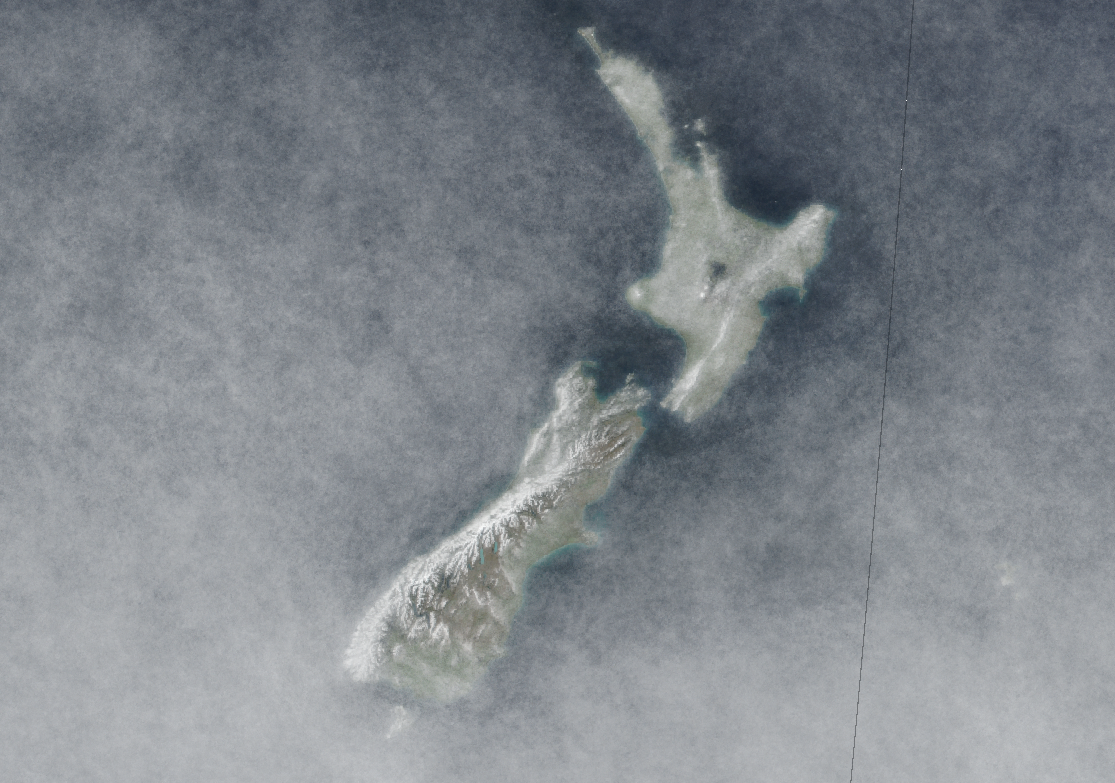
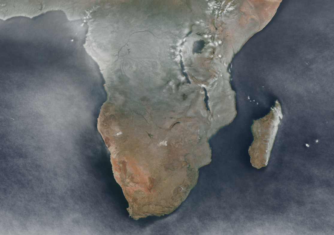
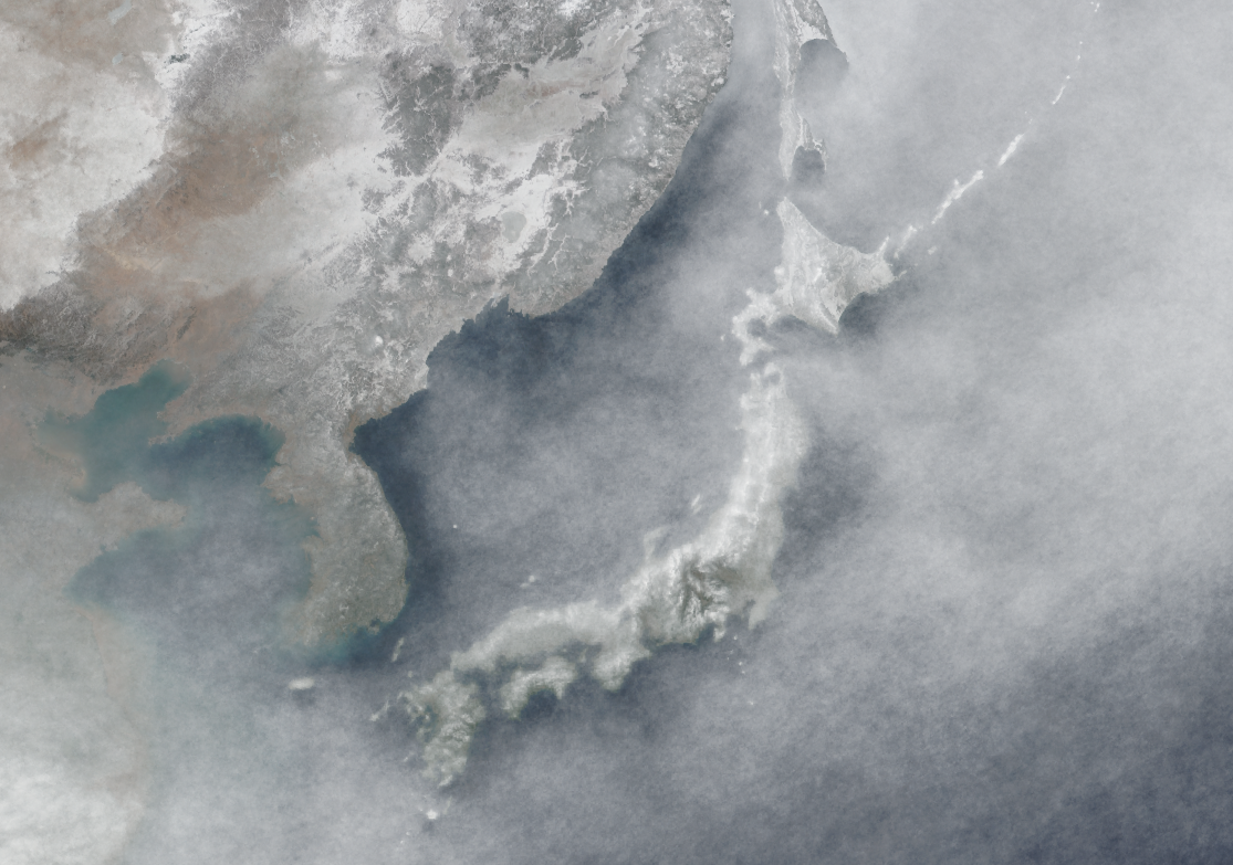
A follow-up to Average Earth from Space 2018 with a how-to. For each day of 2020 I took one global true color image of the whole planet and merged them together by using the most typical color per pixel. You can see cloud patterns in astonishing detail, global wind, permafrost (careful, white can be ice and/or clouds here) and more. Scroll to the bottom for interactive full resolution viewers.


Basically we will want to overlay one satellite image per day into one image for the whole year. You need two things: The images and the GDAL suite of geospatial processing tools.
Imagery
You can get a daily satellite composite of (almost) the whole earth from NASA. For example of the Soumi NPP / VIIRS instrument. Check it out at WorldView.
You can download those images via Global Imagery Browse Services (GIBS).
As the API I used two years ago is gone, Joshua Stevens was so nice to share code he used previously. It was easy to adapt:
set -e
set -u

# run like: $ bash gibs_viirs.sh 2020-10-05
# you get: VIIRS_SNPP_CorrectedReflectance_TrueColor-2020-10-05.tif
# in ~15 minutes and at ~600 megabytes for 32768x16384 pixels

# based on https://gist.github.com/jscarto/6c0413f4820ed5141744e96e19f31205

# https://gibs.earthdata.nasa.gov/wmts/epsg4326/best/1.0.0/WMTSCapabilities.xml
# VIIRS_SNPP_CorrectedReflectance_TrueColor is not served as PNG by GIBS
# so this is using JPEG tiles as source

# -outsize 65536 32768 took ~50 minutes
# -outsize 32768 16384 took ~15 minutes
# you can run multiple instances at once without issues to reduce total time

# TODO probably should be using a less detailed tileset than 250m to put
# less stress on the server...!

layer=VIIRS_SNPP_CorrectedReflectance_TrueColor
caldate=$1  # 2020-09-09
tilelevel=8  # 8 is the highest for 250m, see Capa -> 163840 81920 would be the full outsize
# 2022 says: Dude, check what gdal says for "Input file size is x, y" and then compare it to the outsize. Use the tilelevel that gives 2x the outsize, that seems to be what's needed

# ready? let's go!
gdal_translate \
-outsize 32768 16384 \
-projwin -180 90 180 -90 \
-of GTIFF \
-co TILED=YES \
-co COMPRESS=DEFLATE \
-co PREDICTOR=2 \
-co NUM_THREADS=ALL_CPUS \
"<GDAL_WMS>
 <Service name=\"TMS\">
 <ServerUrl>https://gibs.earthdata.nasa.gov/wmts/epsg4326/best/"${layer}"/default/"${caldate}"/250m/\${z}/\${y}/\${x}.jpg</ServerUrl>
</Service>
<DataWindow>
 <UpperLeftX>-180.0</UpperLeftX><!-- makes sense -->
 <UpperLeftY>90</UpperLeftY><!-- makes sense -->
 <LowerRightX>396.0</LowerRightX><!-- wtf -->
 <LowerRightY>-198</LowerRightY><!-- wtf -->
 <TileLevel>"${tilelevel}"</TileLevel>
 <TileCountX>2</TileCountX>
 <TileCountY>1</TileCountY>
 <YOrigin>top</YOrigin>
</DataWindow>
<Projection>EPSG:4326</Projection>
<BlockSizeX>512</BlockSizeX><!-- correct for VIIRS_SNPP_CorrectedReflectance_TrueColor-->
<BlockSizeY>512</BlockSizeY><!-- correct for VIIRS_SNPP_CorrectedReflectance_TrueColor -->
<BandsCount>3</BandsCount>
</GDAL_WMS>" \
${layer}-${caldate}.tif
As this was no scientific project, please note that I have spent no time checking e. g.:
- If one could reduce the (significantly) compression artifacts of imagery received through this (the imagery is only provided as JPEG using this particular API),
- if the temporal queries are actually getting the correct dates,
- if there might be more imagery available
- or even if the geographic referencing is correct.
As it takes a long time to fetch an image this way, I decided to go for a resolution of 32768×16384 pixels instead of 65536×32768 because the latter took about 50 minutes per image. A day of 32768×16384 pixels took me about 15 minutes to download.
Overlaying the images
There are lots of options to overlay images. imagemagick/graphicsmagick might be the obvious choice but they are unfit for imagery of these dimensions (exhausting RAM). VIPS/nips2 is awesome but might require some getting used to and/or manual processing. GDAL is the hot shit and very RAM friendly if you are careful. So I used GDAL for this.
Make sure to store the images somewhere sensible for lots of I/O.
Got all the images you want to process? Cool, build a VRT for them:
gdalbuildvrt \
VIIRS_SNPP_CorrectedReflectance_TrueColor-2020.vrt \
VIIRS_SNPP_CorrectedReflectance_TrueColor-2020-*.tif
This takes some seconds.
We want to overlay the images with some fancy, highly complex mathematical formula (or not ;) ) and since GDAL’s VRT driver supports custom Python functions to manipulate pixel values, we can use numpy for that. Put this in a file called functions.py and remember the path to that file:
import numpy as np

def median(in_ar, out_ar, xoff, yoff, xsize, ysize, raster_xsize,
      raster_ysize, buf_radius, gt,  **kwargs):
    out_ar[:] = np.median(in_ar, axis = 0)

def mean(in_ar, out_ar, xoff, yoff, xsize, ysize, raster_xsize,
      raster_ysize, buf_radius, gt,  **kwargs):
    out_ar[:] = np.mean(in_ar, axis = 0)

def max(in_ar, out_ar, xoff, yoff, xsize, ysize, raster_xsize,
      raster_ysize, buf_radius, gt,  **kwargs):
    out_ar[:] = np.amax(in_ar, axis = 0)

def min(in_ar, out_ar, xoff, yoff, xsize, ysize, raster_xsize,
      raster_ysize, buf_radius, gt,  **kwargs):
    out_ar[:] = np.amin(in_ar, axis = 0)
You can now use a median, mean, min or max function for aggregating the images per pixel. For that you have to modify the VRT to include the function you want it to use. I used sed for that:
sed -e 's#<VRTRasterBand#<VRTRasterBand subClass="VRTDerivedRasterBand"#' \
-e 's#</ColorInterp>#</ColorInterp>\n<PixelFunctionLanguage>Python</PixelFunctionLanguage>\n<PixelFunctionType>functions.median</PixelFunctionType>#' \
VIIRS_SNPP_CorrectedReflectance_TrueColor-2020.vrt \
> VIIRS_SNPP_CorrectedReflectance_TrueColor-2020_median.vrt
That’s it, we are ready to use GDAL to build an image that combines all the daily images into one median image. For this to work you have to set the PYTHONPATH environment variable to include the directory of the functions.py file. If it is in the same directory where you launch gdal, you can use $PWD, otherwise enter the full path to the directory. Adjust the rest of the options as you like, e. g. to choose a different output format. If you use COG, enabling ALL_CPUS is highly recommended or building overviews will take forever.
PYTHONPATH=$PWD gdal_translate \
--config CPL_DEBUG VRT --config GDAL_CACHEMAX 25% \
--config GDAL_VRT_ENABLE_PYTHON YES \
-of COG -co NUM_THREADS=ALL_CPUS \
-co COMPRESS=DEFLATE -co PREDICTOR=2 \
VIIRS_SNPP_CorrectedReflectance_TrueColor-2020_median.vrt \
VIIRS_SNPP_CorrectedReflectance_TrueColor-2020_median.vrt.tif
This will take many hours. 35 hours for me on a Ryzen 3600 with lots of RAM and the images on a cheap SSD. The resulting file is about the same size as the single images (makes sense, doesn’t it) at ~800 megabytes.
Alternative, faster approach
A small note while we are at it: GDAL calculates overviews from the source data. And since we are using a custom VRT function here, on a lot of raster images, that takes a long time. To save a lot of that time, you can build the file without overviews first, then calculate them in a second step. With this approach they will be calculated from the final raster instead of the initial input which, when ever there is non-trivial processing involved, is way quicker:
PYTHONPATH=$PWD gdal_translate \
--config CPL_DEBUG VRT --config GDAL_CACHEMAX 25% \
--config GDAL_VRT_ENABLE_PYTHON YES \
-of GTiff -co NUM_THREADS=ALL_CPUS \
VIIRS_SNPP_CorrectedReflectance_TrueColor-2020_median.vrt \
VIIRS_SNPP_CorrectedReflectance_TrueColor-2020_median.vrt.noovr.tif
Followed by the conversion to a COG (which automatically will build the overviews as mandatory for that awesome format):
gdal_translate \
--config GDAL_CACHEMAX 25% \
-of COG -co NUM_THREADS=ALL_CPUS \
-co COMPRESS=DEFLATE -co PREDICTOR=2 \
/tmp/VIIRS_SNPP_CorrectedReflectance_TrueColor-2020_median.vrt.noovr.tif \
VIIRS_SNPP_CorrectedReflectance_TrueColor-2020_median.vrt.cog.tif
This took “just” 10 hours for the initial raster and then an additional 11 seconds for the conversion COG and the building of overviews. And the resulting file is bit-by-bit identical to the one from the direct-to-COG approach. So one third of processing time for the same result. Nice!
Result
Check it out in full, zoomable resolution:
- EPSG:4326 1:1 to the data I used via geotiffjs.github.io
- Pseudo/Web Mercator EPSG:3857 using client-side reprojection via cogeo.org
Or download the Cloud-Optimized GeoTIFF file for your own software:
- EPSG:4326 (800MB)


Closing remarks
Please do not consider a true representation of the typical weather or cloud cover throughout the year. The satellite takes the day imagery at local noon if I recall correctly so the rest of the day is not part of this “analysis”. I did zero plausibility or consistency checks. The data was probably reprojected multiple times through out the full (sensor->composite) pipeline. The composite is based on color alone, anything bright will lead to a white-ish color, be it snow, ice, clouds, algae, sand, …
It’s just some neat imagery to love our planet.
Update 2020-01-05
Added compression to GeoTIFF creation where useful, not sure how I missed that here. Reduces filesizes to 1/2 or 1/3 even.
am trying to implement the merge of overlapping functions by taking the median of tif files. I have a vrt file and trying to implement the median pixel function.
median
Python
Reproject6.tif
1
Reproject4.tif
1
Reproject1.tif
1
The out put is not as expected. I would be grateful if anyone could help.
If you left any information that would help pinpointing your problem, then maybe someone could help…
That is so awesome!! I do not understand the entire process though and just wanted to ask if there is any chance to increase the download speed? Maybe lower the resolution of 250 m to some other value (I tried but I am not sure where I can find the values the wmts endpoint accepts).
Anyways, thank you very very much!!
Or is there maybe the chance to pass something like a bounding box, so that it does not query data from the entire earth?:)
Horrible to use, isn’t it? :(
For speeding it up at the cost of resolution you can reduce the outsize to e.g. `-outsize 4096 2048`. Choosing a bounding box is definitely possible but I see my “wtf” comments in he WMTS service definition above and will just walk away again now, sorry.
haha yes, I tried to modify some of these values, but ended up downloading everything…;)
Anyways, thank you very much again! This is pretty awesome
Pingback: Average Earth from Space 2018 | Hannes ihm sein Blog