NOTE: In up to date GDAL things might be easier AND I messed up with --config and -co below. Poke me to update it please.
So about half a year ago Lukas Martinelli asked about a global SRTM GeoTIFF. The SRTM elevation data is usually shared in many small tiles which can be ideal for some cases but annoying for others. I like downloading and processing big files so I took that as a challenge. It’s probably some mental thing. I never finished this blog post back then. It’s probably another mental thing. 8) Read on if you are interested in some GNU coreutils hackery as well as GDAL magick.
Zooming through a live-hillshaded global SRTMGL1 30m GeoTIFF (130GB) in #QGIS (ok, sped up 2x but still awesome). pic.twitter.com/5nwWdlBx7o
— cartocalypse (@cartocalypse) October 2, 2016
Here is how I did it. Endless thanks as usual to Even Rouault who fixed GDAL bugs and gave great hints. I learned more about GeoTIFFs and GDAL than I should have needed to know.
Downloading the source files
The source files are available at http://e4ftl01.cr.usgs.gov/SRTM/SRTMGL1.003/2000.02.11/ (warning, visiting this URL will make your browser cry and potentially render your system unresponsive). To download them you must create an NASA Earthdata Login at https://urs.earthdata.nasa.gov/users/new/. :\
********************************************************************************

                         U.S. GOVERNMENT COMPUTER

This US Government computer is for authorized users only.  By accessing this
system you are consenting to complete monitoring with no expectation of privacy.
Unauthorized access or use may subject you to disciplinary action and criminal
prosecution.
OMGOMGOMG. I am sure they would have used <blink> if accessibility guidelines allowed it. As I am not sure what their Terms of Service are, I will not give you a copy’n’paste ready line to download them all. wget or aria2 work well. You should get 14297 files with a total size of 98G.
Inspecting the ZIP files and preparing for GDAL’s vsizip
Each of those ZIP files has just a single file “.hgt” inside. GDAL specifically has support for the “SRTM HGT Format“, so we know it can read those files. We just need to extract them. (If you clicked that link you see that with GDAL 2.2 it will support directly loading the data from the ZIPs, that’s just Even being awesome.)
We don’t want to uncompress all those files just because we want to build a GeoTIFF from them later, do we? Luckily GDAL has a vsizip thingie which allows it to read files inside zip archives. Wicked! For this we need the “deep” paths to the files though, for example e4ftl01.cr.usgs.gov/SRTM/SRTMGL1.003/2000.02.11/N29E000.SRTMGL1.hgt.zip/N29E000.hgt.
The files inside the archives are always simply the same filename minus the “.SRTMGL1” and the .zip extension. Perfect, now we know all the files from inside the ZIPs! Right? Nope. Unfortunately some (17) of the archives do include the “.SRTMGL1” bit in their files, for example N38E051.SRTMGL1.hgt… >:(
That’s why we need to look into each zip file and determine the filename inside. (Alternatively *you* could extract them all after all, you with your fancy, huge SSD.)
We can simply use `unzip` with the `-t` switch to make it show what’s inside (and as a “free” benefit it will also check the file’s integrity for us). `tee` is used here to save the output to a file. This will take a while as it needs to read through all the files…
$ unzip -t "e4ftl01.cr.usgs.gov/SRTM/SRTMGL1.003/2000.02.11/*.SRTMGL1.hgt.zip" | tee unzip-t.log
...

Archive: e4ftl01.cr.usgs.gov/SRTM/SRTMGL1.003/2000.02.11/N29E000.SRTMGL1.hgt.zip
testing: N29E000.hgt OK
No errors detected in compressed data of e4ftl01.cr.usgs.gov/SRTM/SRTMGL1.003/2000.02.11/N29E000.SRTMGL1.hgt.zip.

Archive: e4ftl01.cr.usgs.gov/SRTM/SRTMGL1.003/2000.02.11/N27E033.SRTMGL1.hgt.zip
testing: N27E033.hgt OK
No errors detected in compressed data of e4ftl01.cr.usgs.gov/SRTM/SRTMGL1.003/2000.02.11/N27E033.SRTMGL1.hgt.zip.

Archive: e4ftl01.cr.usgs.gov/SRTM/SRTMGL1.003/2000.02.11/N45E066.SRTMGL1.hgt.zip
testing: N45E066.hgt OK
No errors detected in compressed data of e4ftl01.cr.usgs.gov/SRTM/SRTMGL1.003/2000.02.11/N45E066.SRTMGL1.hgt.zip.

14297 archives were successfully processed.
14297 archives were successfully processed.
Yay, no errors!
In the output we see the path to the archive and we see the name of the file inside. With some sed and grep we can easily construct “deep” paths.
First we remove the status lines, the blank lines and the very last full status line with `grep`:
$ cat unzip-t.log | grep -v -e "No errors" -e '^$' -e 'successfully processed'
Archive: e4ftl01.cr.usgs.gov/SRTM/SRTMGL1.003/2000.02.11/N12E044.SRTMGL1.hgt.zip
testing: N12E044.hgt OK
Archive: e4ftl01.cr.usgs.gov/SRTM/SRTMGL1.003/2000.02.11/N29W002.SRTMGL1.hgt.zip
testing: N29W002.hgt OK
Archive: e4ftl01.cr.usgs.gov/SRTM/SRTMGL1.003/2000.02.11/N45E116.SRTMGL1.hgt.zip
testing: N45E116.hgt OK
Then we concatenate every consecutive two lines into one line with `paste` (I LOVE THIS 1 TRICK!):
$ cat unzip-t.log | grep -v -e "No errors" -e '^$' -e 'successfully processed' | paste - -
Archive: e4ftl01.cr.usgs.gov/SRTM/SRTMGL1.003/2000.02.11/N12E044.SRTMGL1.hgt.zip testing: N12E044.hgt OK
Archive: e4ftl01.cr.usgs.gov/SRTM/SRTMGL1.003/2000.02.11/N29W002.SRTMGL1.hgt.zip testing: N29W002.hgt OK
Archive: e4ftl01.cr.usgs.gov/SRTM/SRTMGL1.003/2000.02.11/N45E116.SRTMGL1.hgt.zip testing: N45E116.hgt OK
Finally we strip things away with sed (I don’t care that you would do it differently, this is how I quickly did it with my flair of hammering) and direct the output into a new file called `zips`:
$ cat unzip-t.log | grep -v -e "No errors" -e '^$' -e 'successfully processed' | paste - - | sed -e 's#Archive:[ ]*##' -e 's#\t[ ]*testing: #/#' -e 's#[ ]*OK##' > zips
e4ftl01.cr.usgs.gov/SRTM/SRTMGL1.003/2000.02.11/N12E044.SRTMGL1.hgt.zip/N12E044.hgt
e4ftl01.cr.usgs.gov/SRTM/SRTMGL1.003/2000.02.11/N29W002.SRTMGL1.hgt.zip/N29W002.hgt
e4ftl01.cr.usgs.gov/SRTM/SRTMGL1.003/2000.02.11/N45E116.SRTMGL1.hgt.zip/N45E116.hgt
Yay, we have all the actual inside-zip paths now!
If you are curious, you can try gdalinfo with those now. You need to prepend /vsizip/ to the path to make it read inside zip files.
$ gdalinfo /vsizip/e4ftl01.cr.usgs.gov/SRTM/SRTMGL1.003/2000.02.11/N12E044.SRTMGL1.hgt.zip/N12E044.hgt
Driver: SRTMHGT/SRTMHGT File Format
Files: /vsizip/e4ftl01.cr.usgs.gov/SRTM/SRTMGL1.003/2000.02.11/N12E044.SRTMGL1.hgt.zip/N12E044.hgt
Size is 3601, 3601
Coordinate System is:
GEOGCS["WGS 84",
    DATUM["WGS_1984",
        SPHEROID["WGS 84",6378137,298.257223563,
            AUTHORITY["EPSG","7030"]],
        AUTHORITY["EPSG","6326"]],
    PRIMEM["Greenwich",0,
        AUTHORITY["EPSG","8901"]],
    UNIT["degree",0.0174532925199433,
        AUTHORITY["EPSG","9122"]],
    AUTHORITY["EPSG","4326"]]
Origin = (43.999861111111109,13.000138888888889)
Pixel Size = (0.000277777777778,-0.000277777777778)
Metadata:
  AREA_OR_POINT=Point
Corner Coordinates:
Upper Left  (  43.9998611,  13.0001389) ( 43d59'59.50"E, 13d 0' 0.50"N)
Lower Left  (  43.9998611,  11.9998611) ( 43d59'59.50"E, 11d59'59.50"N)
Upper Right (  45.0001389,  13.0001389) ( 45d 0' 0.50"E, 13d 0' 0.50"N)
Lower Right (  45.0001389,  11.9998611) ( 45d 0' 0.50"E, 11d59'59.50"N)
Center      (  44.5000000,  12.5000000) ( 44d30' 0.00"E, 12d30' 0.00"N)
Band 1 Block=3601x1 Type=Int16, ColorInterp=Undefined
  NoData Value=-32768
  Unit Type: m
Hooray! GDAL reads the hgt file from inside its zip!
We need to prepend all the paths with `/vsizip/` so let’s do that:
$ sed 's#^#/vsizip/##' zips > vsizips
/vsizip/e4ftl01.cr.usgs.gov/SRTM/SRTMGL1.003/2000.02.11/N12E044.SRTMGL1.hgt.zip/N12E044.hgt
/vsizip/e4ftl01.cr.usgs.gov/SRTM/SRTMGL1.003/2000.02.11/N29W002.SRTMGL1.hgt.zip/N29W002.hgt
/vsizip/e4ftl01.cr.usgs.gov/SRTM/SRTMGL1.003/2000.02.11/N45E116.SRTMGL1.hgt.zip/N45E116.hgt
Unfortunately those 17 misnamed files from earlier need special treatment… This is what my notes say, not sure what it was supposed to do. If you are recreating this all, please just ask me and I will look at it again. For now, let’s just pretend that this leads to a file called `hgtfiles` in which all the paths are perfect and all the files are perfect.
grep -v 'SRTMGL1.hgt$' vsizips > vsizipswithoutmisnamedfiles

mkdir misnamedfiles

cd misnamedfiles/

nano ../listofmisnamedfiles # insert the paths to those 17 zips here #TODO

while read filename; do unzip "../${filename}"; done < ../listofmisnamedfiles

rename 's/SRTMGL1.//' *.hgt

cd ..

find misnamedfiles/ -type f > listofmisnamedfileshgt

cat listofmisnamedfileshgt vsizipswithoutmisnamedfiles > hgtfiles
As I said above though, go with a recent GDAL and this is all much easier. Even even included a check for the different filenames inside, how can you not like that guy!
Building a Virtual Raster Table
Virtual Raster Tables (VRT) are some kind of files that pretend to be rasters. They are awesome. Here we use a VRT that simply turns all the small rasters we have into one big ass raster.
Ok, ready to create a Virtual Raster Table!
$ time gdalbuildvrt -input_file_list hgtfiles srtmgl1.003.vrt
0...10...20...30...40...50...60...70...80...90...100 - done.

real 0m22.679s
user 0m19.250s
sys 0m3.105s
Done.
You could go ahead and use this for your work/leisure now. But remember, it is tens of gigabytes of data so if you do not use it at a 1:1 scale things will not be fun and might fry your cat. You want overviews/pyramids.
Turning the VRT into a GeoTIFF (Optional)
Let’s make a HUGEGEOTIFF because that’s cool! You don’t have to, instead you could build overviews for the .vrt file.
We want it quick to read and small so I used DEFLATE, TILED and the horizontal predictor. I ran this on a weak i7 with 2G of RAM and can’t remember what the worst bottleneck was. Probably CPU.
$ time gdal_translate -co NUM_THREADS=ALL_CPUS --config PREDICTOR 2 -co COMPRESS=DEFLATE -co TILED=YES -co BIGTIFF=YES srtmgl1.003.vrt srtmgl1.003.vrt.tif
Input file size is 1296001, 417601
0...10...20...30...40...50...60...70...80...90...100 - done.

real 231m57.961s
user 503m23.044s
sys 3m14.600s
If you are courageous you can load that file in your GIS now. But again, unless you watch it at a 1:1 scale or something close to that it WILL not be much fun and potentially expose weaknesses in your GIS and fill up your system’s memory and crash and you had no unsaved work open, didn’t you?
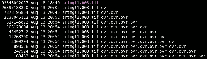
Building Overviews
Overviews aka pyramids are usually about 1/3 the size of the full image. If they are not, you probably used different compression settings. This was the step that I expected to be just boring to wait for, but it turned out the most problematic. I tried all available free tools but none worked properly with an input this big. With GDAL we found a workaround after a while.
gdaladdo has problems building multiple overview levels with a file this big… The trick is to built the overviews sequentially, not in one invocation. The best solution at the moment was building overviews for overviews for overviews and so on until you reach a comfortable size. Something like:
gdaladdo -ro srtmgl1.003.tif 2

gdaladdo -ro srtmgl1.003.tif.ovr 2

gdaladdo -ro srtmgl1.003.tif.ovr.ovr 2

gdaladdo -ro srtmgl1.003.tif.ovr.ovr.ovr 2

gdaladdo -ro srtmgl1.003.tif.ovr.ovr.ovr.ovr 2 4 8 16 32 64 128 256 512
I used the following parameters:
gdaladdo -oo NUM_THREADS=ALL_CPUS --config GDAL_NUM_THREADS ALL_CPUS --config GDAL_CACHEMAX 2048 --config COMPRESS_OVERVIEW DEFLATE --config PREDICTOR_OVERVIEW 2 --config BIGTIFF_OVERVIEW YES -ro
Apparently gdaladdo automatically makes them tiled, which is good. I used https://gist.github.com/springmeyer/3007985 to find out.
Creating overviews took just about 3 hours with this weird trick. So, in total the processing just takes half a day.
Download
Enjoy! https://www.datenatlas.de/geodata/public/srtmgl1/. I impose no license/copyright/whatever on this derivative work.
TODO
Hillshading? Slope? You do it!
Found a better, faster way? You blog it!
We could add the overviews to the main image with `gdal_translate srtmgl1.003.tif srtmgl1.003.withovr.tif -co COPY_SRC_OVERVIEWS=YES [other options]` says Even.


