Category Archives: gdal

The effect of lossy LERC compression, visually “explained”

LERC is a kick-ass approach to 2D raster data compression, supported in GDAL since version 3.3. You can use it for lossless compression but it is also able to throw away some bits of information for smaller data sizes. You tell it which level of Z error is acceptable for your values and it will use that freedom to change the values of neighboring cells to do its magic. Z means the “data” axis here, of a single-band in a 2D raster, X and Y are the coordinates, or rather the locations of the data values in the raster, which are obviously not changed.

I thought it would be nice to show what it actually results in, you can read up on the details elsewhere if you want. Look at the images in full resolution please.

I used a global SRTM DEM with a Z value in full meters (no floating point values but integers) and applied LERC on it in three ways: Lossless, with a maximum Z error of 1 meter and a maximum Z error of 10 meters. Zstandard compression was always used.

The original GeoTIFF file was already very well compressed with Zstandard level 15 and a horizontal predictor; at ~1296000 x ~417600 pixels it has a size of 86 gigabytes including overviews.

  • Original (ZSTD level 15): 86 GB
  • LERC_ZSTD (lossless): 105G
  • LERC_ZSTD (maximum Z error of 1): 81G
  • LERC_ZSTD (maximum Z error of 10): 21G

Cool, so if we don’t care about an error of 10 meters, we can have a global DEM (well, as global as SRTM is with its 60° cut-off) at ~30 meters pixel resolution in 21 gigabytes. But what does that actually look like then and how will this error appear? Well, check it out:

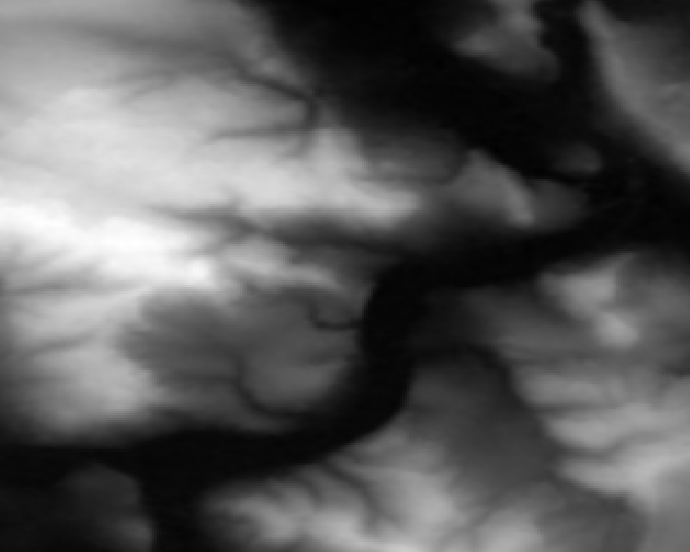
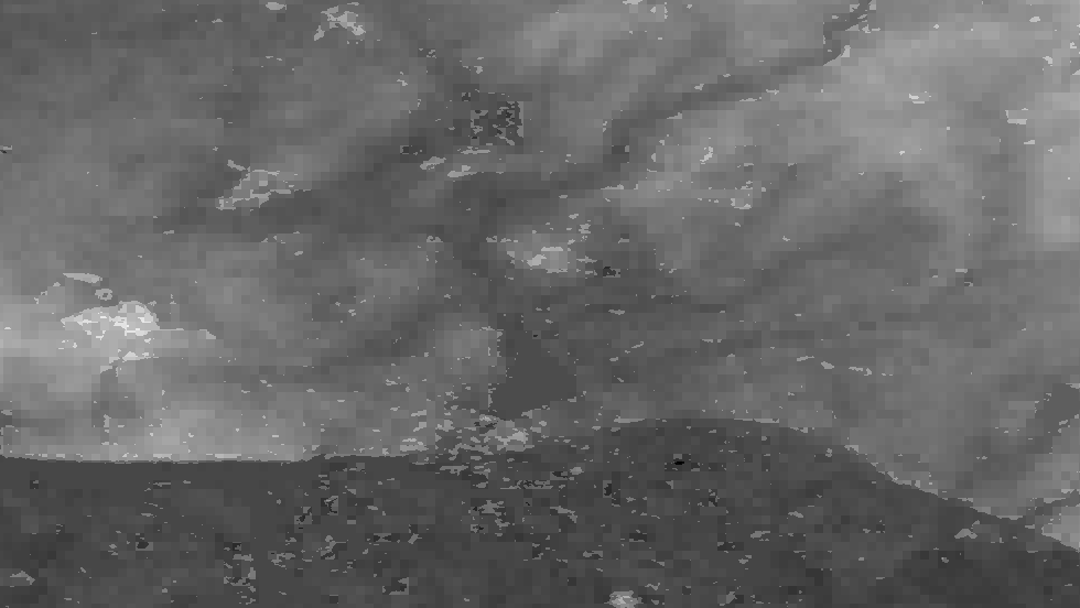
Here are some samples visualised with a greyscale color ramp (locally adjusted, so the lowest value in the image is black, the highest value is white). They are shown at a 1:1 resolution, one pixel in the image (if you look at it at 100%) is one cell of the DEM data. The left image is lossless, the middle one was allowed an Z error of 1 meter, the right one 10 meters.

Mountainous, here the values range from 0 meters to about 2000 meters:

You can hardly see a difference, at least visually.

“Mediumish”, values between ~100 and ~500 meters:

At the 10 meter error level you can see a significant terracing effect.

Plains, values all around 100 meters:

You can see some structures collapsing into flat areas in the 1 meter version and oh wow that 10 meters version looks like upscaled pixels.

Time to zoom in! I picked a less flat area again because it makes it easier to understand. Here the values are between ~100 and ~300 meters:

So what do we see here? Neighboring cells with the same values compress better so LERC is shifting the values around (within the allowed error), creating terraces of same-valued cells. If you look closely you can see that there is also a visible pattern of squarish structures. Those are the blocks or windows in which LERC looks at the data and does its adjustments, in this case they were 8×8 pixels wide. Note: What LERC does exactly is a bit more complex than “try to make neighboring values the same”, it actually looks at the bits required to store the values within a block and optimized that within the error tolerance.

And now you know what LERC can do, if you give it a error level to play with.

For reference, here is that same-ish area with the error tolerance at 1 meter:

You have to zoom in quite a bit more to be able to see the effects here due to the nature of the data in this extent in combination with the particular error tolerance:

The larger the zonal differences of your Z values are to each other and in relation to the error tolerance, the less distinguished will this effect be. If there are steps of 100 meters between neighboring pixels, an extra error of 10 meters won’t do much of a difference. But in more flat areas it will have significant “terracing” effects as you could see above. This is similar to “banding” effects in images where there is little variation in color, e. g. a blue sky or an artificial color gradient, and you look at it in a setup that has a color bit depth on a resolution your human eyes can distinguish.

So if you want to use LERC with a lossy approach, think hard about what is going to happen with your data later. What kind of analysis will be performed, how will it be “looked” at, what will be calculated. Do it smart and you can have a predictable/controllable lossy compression with seriously small file sizes, do it without thinking and your data will lead to misinterpretation and apocalypse.

Satellite composite of Earth 2020

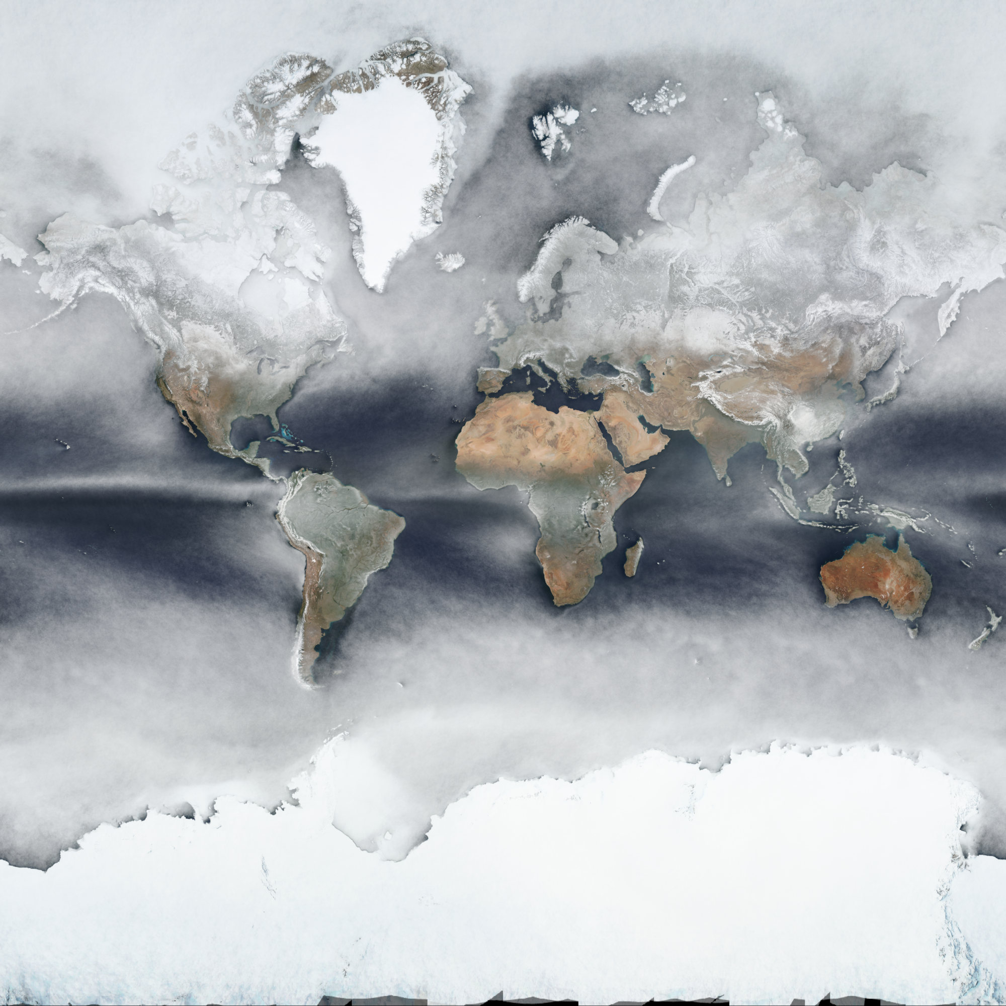
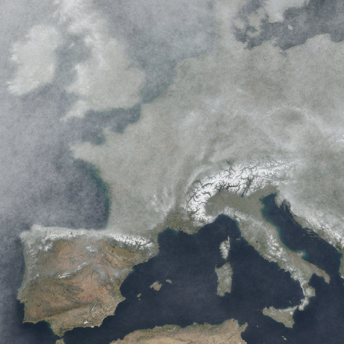
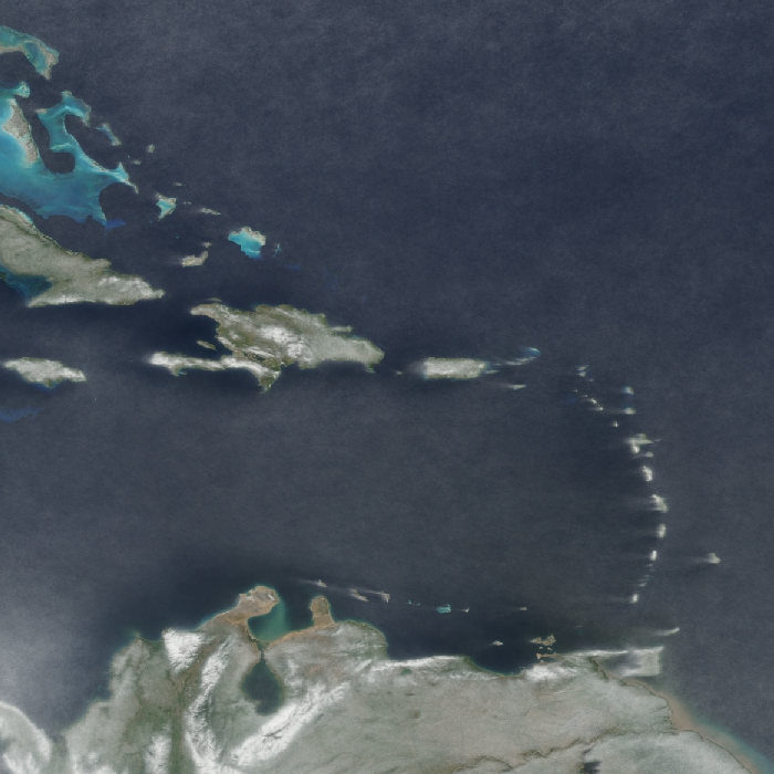
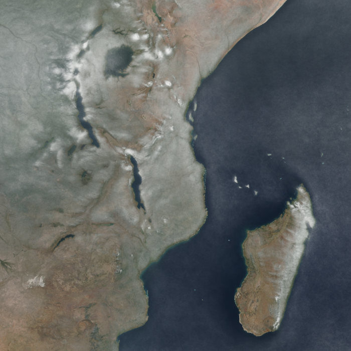
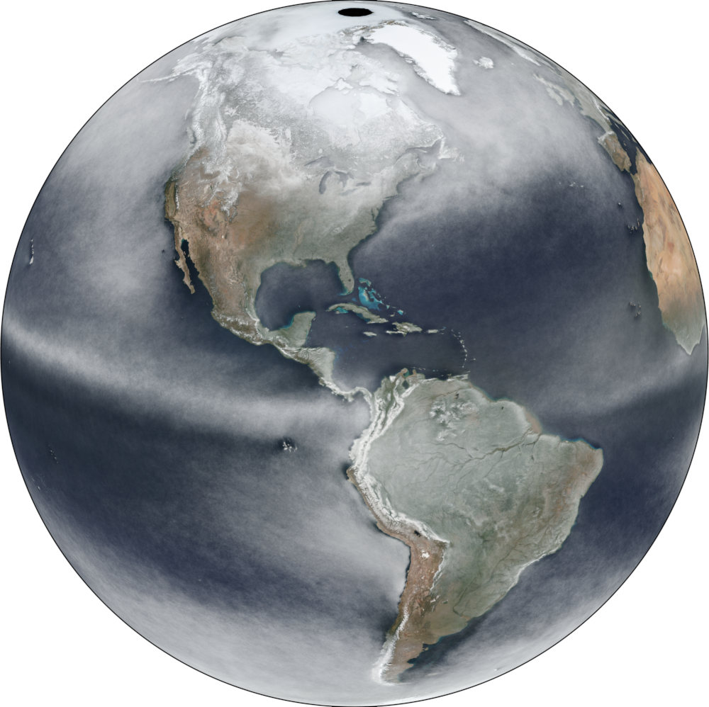
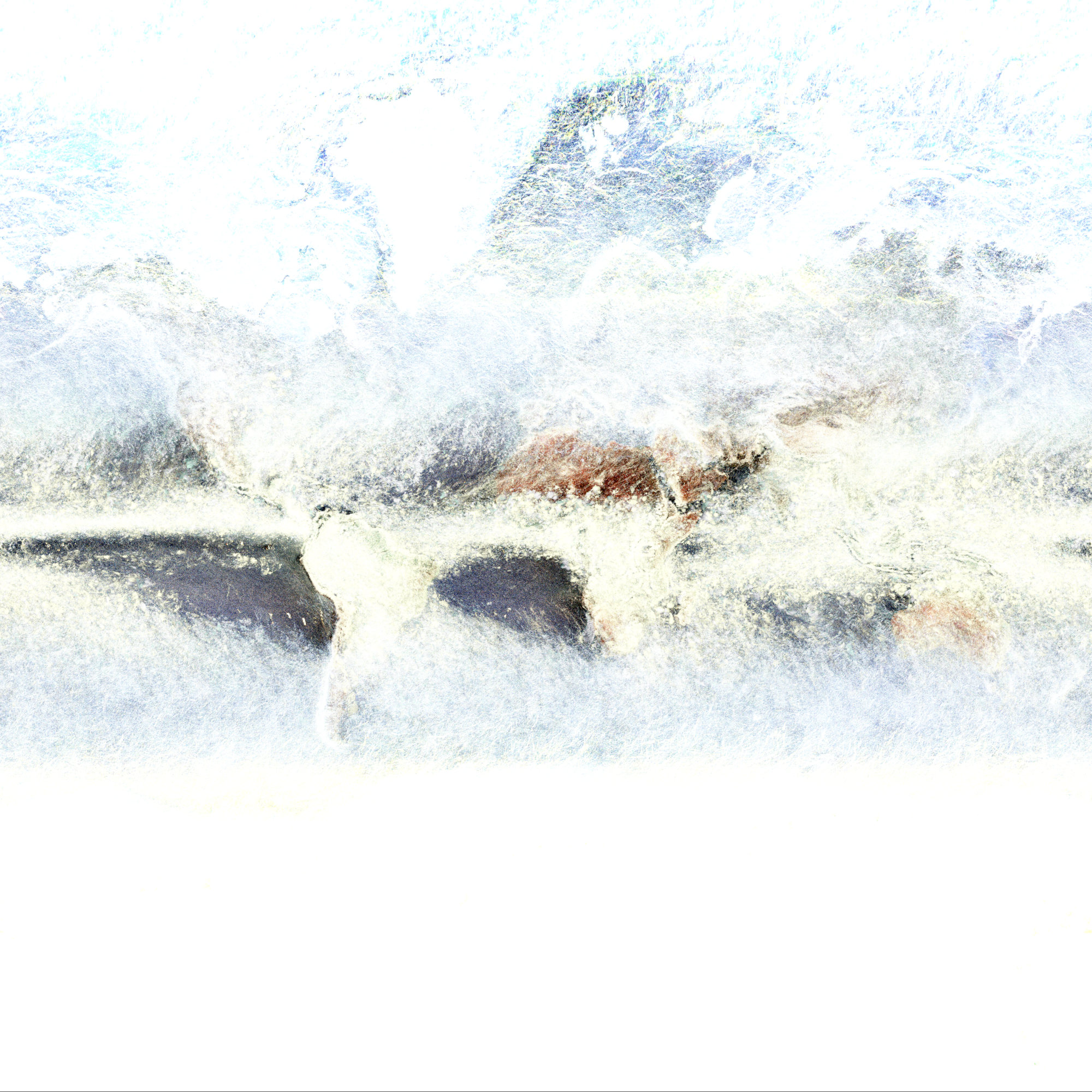
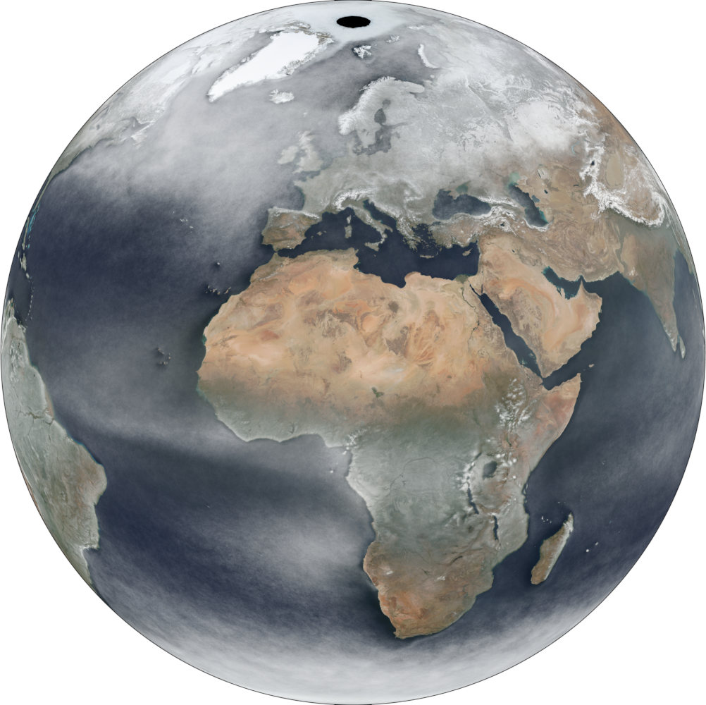
A follow-up to Average Earth from Space 2018 with a how-to. For each day of 2020 I took one global true color image of the whole planet and merged them together by using the most typical color per pixel. You can see cloud patterns in astonishing detail, global wind, permafrost (careful, white can be ice and/or clouds here) and more. Scroll to the bottom for interactive full resolution viewers.

Basically we will want to overlay one satellite image per day into one image for the whole year. You need two things: The images and the GDAL suite of geospatial processing tools.

Imagery

You can get a daily satellite composite of (almost) the whole earth from NASA. For example of the Soumi NPP / VIIRS instrument. Check it out at WorldView.

You can download those images via Global Imagery Browse Services (GIBS).

As the API I used two years ago is gone, Joshua Stevens was so nice to share code he used previously. It was easy to adapt:

set -e
set -u

# run like: $ bash gibs_viirs.sh 2020-10-05
# you get: VIIRS_SNPP_CorrectedReflectance_TrueColor-2020-10-05.tif
# in ~15 minutes and at ~600 megabytes for 32768x16384 pixels

# based on https://gist.github.com/jscarto/6c0413f4820ed5141744e96e19f31205

# https://gibs.earthdata.nasa.gov/wmts/epsg4326/best/1.0.0/WMTSCapabilities.xml
# VIIRS_SNPP_CorrectedReflectance_TrueColor is not served as PNG by GIBS
# so this is using JPEG tiles as source

# -outsize 65536 32768 took ~50 minutes
# -outsize 32768 16384 took ~15 minutes
# you can run multiple instances at once without issues to reduce total time

# TODO probably should be using a less detailed tileset than 250m to put
# less stress on the server...!

layer=VIIRS_SNPP_CorrectedReflectance_TrueColor
caldate=$1  # 2020-09-09
tilelevel=8  # 8 is the highest for 250m, see Capa -> 163840 81920 would be the full outsize
# 2022 says: Dude, check what gdal says for "Input file size is x, y" and then compare it to the outsize. Use the tilelevel that gives 2x the outsize, that seems to be what's needed

# ready? let's go!
gdal_translate \
-outsize 32768 16384 \
-projwin -180 90 180 -90 \
-of GTIFF \
-co TILED=YES \
-co COMPRESS=DEFLATE \
-co PREDICTOR=2 \
-co NUM_THREADS=ALL_CPUS \
"<GDAL_WMS>
 <Service name=\"TMS\">
 <ServerUrl>https://gibs.earthdata.nasa.gov/wmts/epsg4326/best/"${layer}"/default/"${caldate}"/250m/\${z}/\${y}/\${x}.jpg</ServerUrl>
</Service>
<DataWindow>
 <UpperLeftX>-180.0</UpperLeftX><!-- makes sense -->
 <UpperLeftY>90</UpperLeftY><!-- makes sense -->
 <LowerRightX>396.0</LowerRightX><!-- wtf -->
 <LowerRightY>-198</LowerRightY><!-- wtf -->
 <TileLevel>"${tilelevel}"</TileLevel>
 <TileCountX>2</TileCountX>
 <TileCountY>1</TileCountY>
 <YOrigin>top</YOrigin>
</DataWindow>
<Projection>EPSG:4326</Projection>
<BlockSizeX>512</BlockSizeX><!-- correct for VIIRS_SNPP_CorrectedReflectance_TrueColor-->
<BlockSizeY>512</BlockSizeY><!-- correct for VIIRS_SNPP_CorrectedReflectance_TrueColor -->
<BandsCount>3</BandsCount>
</GDAL_WMS>" \
${layer}-${caldate}.tif

As this was no scientific project, please note that I have spent no time checking e. g.:

  • If one could reduce the (significantly) compression artifacts of imagery received through this (the imagery is only provided as JPEG using this particular API),
  • if the temporal queries are actually getting the correct dates,
  • if there might be more imagery available
  • or even if the geographic referencing is correct.

As it takes a long time to fetch an image this way, I decided to go for a resolution of 32768×16384 pixels instead of 65536×32768 because the latter took about 50 minutes per image. A day of 32768×16384 pixels took me about 15 minutes to download.

Overlaying the images

There are lots of options to overlay images. imagemagick/graphicsmagick might be the obvious choice but they are unfit for imagery of these dimensions (exhausting RAM). VIPS/nips2 is awesome but might require some getting used to and/or manual processing. GDAL is the hot shit and very RAM friendly if you are careful. So I used GDAL for this.

Make sure to store the images somewhere sensible for lots of I/O.

Got all the images you want to process? Cool, build a VRT for them:

gdalbuildvrt \
VIIRS_SNPP_CorrectedReflectance_TrueColor-2020.vrt \
VIIRS_SNPP_CorrectedReflectance_TrueColor-2020-*.tif

This takes some seconds.

We want to overlay the images with some fancy, highly complex mathematical formula (or not ;) ) and since GDAL’s VRT driver supports custom Python functions to manipulate pixel values, we can use numpy for that. Put this in a file called functions.py and remember the path to that file:

import numpy as np

def median(in_ar, out_ar, xoff, yoff, xsize, ysize, raster_xsize,
      raster_ysize, buf_radius, gt,  **kwargs):
    out_ar[:] = np.median(in_ar, axis = 0)

def mean(in_ar, out_ar, xoff, yoff, xsize, ysize, raster_xsize,
      raster_ysize, buf_radius, gt,  **kwargs):
    out_ar[:] = np.mean(in_ar, axis = 0)

def max(in_ar, out_ar, xoff, yoff, xsize, ysize, raster_xsize,
      raster_ysize, buf_radius, gt,  **kwargs):
    out_ar[:] = np.amax(in_ar, axis = 0)

def min(in_ar, out_ar, xoff, yoff, xsize, ysize, raster_xsize,
      raster_ysize, buf_radius, gt,  **kwargs):
    out_ar[:] = np.amin(in_ar, axis = 0)

You can now use a median, mean, min or max function for aggregating the images per pixel. For that you have to modify the VRT to include the function you want it to use. I used sed for that:

sed -e 's#<VRTRasterBand#<VRTRasterBand subClass="VRTDerivedRasterBand"#' \
-e 's#</ColorInterp>#</ColorInterp>\n<PixelFunctionLanguage>Python</PixelFunctionLanguage>\n<PixelFunctionType>functions.median</PixelFunctionType>#' \
VIIRS_SNPP_CorrectedReflectance_TrueColor-2020.vrt \
> VIIRS_SNPP_CorrectedReflectance_TrueColor-2020_median.vrt

That’s it, we are ready to use GDAL to build an image that combines all the daily images into one median image. For this to work you have to set the PYTHONPATH environment variable to include the directory of the functions.py file. If it is in the same directory where you launch gdal, you can use $PWD, otherwise enter the full path to the directory. Adjust the rest of the options as you like, e. g. to choose a different output format. If you use COG, enabling ALL_CPUS is highly recommended or building overviews will take forever.

PYTHONPATH=$PWD gdal_translate \
--config CPL_DEBUG VRT --config GDAL_CACHEMAX 25% \
--config GDAL_VRT_ENABLE_PYTHON YES \
-of COG -co NUM_THREADS=ALL_CPUS \
-co COMPRESS=DEFLATE -co PREDICTOR=2 \
VIIRS_SNPP_CorrectedReflectance_TrueColor-2020_median.vrt \
VIIRS_SNPP_CorrectedReflectance_TrueColor-2020_median.vrt.tif

This will take many hours. 35 hours for me on a Ryzen 3600 with lots of RAM and the images on a cheap SSD. The resulting file is about the same size as the single images (makes sense, doesn’t it) at ~800 megabytes.

Alternative, faster approach

A small note while we are at it: GDAL calculates overviews from the source data. And since we are using a custom VRT function here, on a lot of raster images, that takes a long time. To save a lot of that time, you can build the file without overviews first, then calculate them in a second step. With this approach they will be calculated from the final raster instead of the initial input which, when ever there is non-trivial processing involved, is way quicker:

PYTHONPATH=$PWD gdal_translate \
--config CPL_DEBUG VRT --config GDAL_CACHEMAX 25% \
--config GDAL_VRT_ENABLE_PYTHON YES \
-of GTiff -co NUM_THREADS=ALL_CPUS \
VIIRS_SNPP_CorrectedReflectance_TrueColor-2020_median.vrt \
VIIRS_SNPP_CorrectedReflectance_TrueColor-2020_median.vrt.noovr.tif

Followed by the conversion to a COG (which automatically will build the overviews as mandatory for that awesome format):

gdal_translate \
--config GDAL_CACHEMAX 25% \
-of COG -co NUM_THREADS=ALL_CPUS \
-co COMPRESS=DEFLATE -co PREDICTOR=2 \
/tmp/VIIRS_SNPP_CorrectedReflectance_TrueColor-2020_median.vrt.noovr.tif \
VIIRS_SNPP_CorrectedReflectance_TrueColor-2020_median.vrt.cog.tif

This took “just” 10 hours for the initial raster and then an additional 11 seconds for the conversion COG and the building of overviews. And the resulting file is bit-by-bit identical to the one from the direct-to-COG approach. So one third of processing time for the same result. Nice!

Result

Check it out in full, zoomable resolution:

Or download the Cloud-Optimized GeoTIFF file for your own software:

Closing remarks

Please do not consider a true representation of the typical weather or cloud cover throughout the year. The satellite takes the day imagery at local noon if I recall correctly so the rest of the day is not part of this “analysis”. I did zero plausibility or consistency checks. The data was probably reprojected multiple times through out the full (sensor->composite) pipeline. The composite is based on color alone, anything bright will lead to a white-ish color, be it snow, ice, clouds, algae, sand, …

It’s just some neat imagery to love our planet.

Update 2020-01-05

Added compression to GeoTIFF creation where useful, not sure how I missed that here. Reduces filesizes to 1/2 or 1/3 even.

Make sure you actually do use spatial indexes


Ever ran some GIS analysis in QGIS and it took longer than a second? Chances are that your data did not have spatial indexes for QGIS to utilise and that it could have been magnitudes faster.

I realised just today, after years of using QGIS, that it did not automatically create a spatial index when saving a Shapefile. And because of that, lots of GIS stuff I did in the past, involving saving subsets of data to quick’n’dirty Shapefiles, was slower than necessary.

Sadly QGIS does not communicate lack of spatial indexing to the user in any way. I added a feature request to make Processing warn if no indexing is available.

An example: Running ‘Count points in polygon’ on 104 polygons with 223210 points:

  • Points in original GML file: 449 seconds
    • GML is not a format for processing but meant for data transfer, never ever think of using it for anything else
  • Points in ESRI Shapefile: 30 seconds
  • Points in GeoPackage: 3 seconds
  • Points in ESRI Shapefile with spatial index: 3 seconds
    • Same Shapefile as before but this time I had created a .qix index

So yeah, make sure you don’t only use a reasonable format for your data. And also make sure you do actually have an spatial index.

For Shapefiles, look for a .qix or .sbn side-car file somewhere in the heap of files. In QGIS you can create a spatial index for a vector layer either using the “Create spatial index” algorithm in Processing or the button of the same title in the layer properties’ source tab.

PS: GeoPackages always have a spatial index. That’s reason #143 why they are awesome.

Average Earth from Space 2018

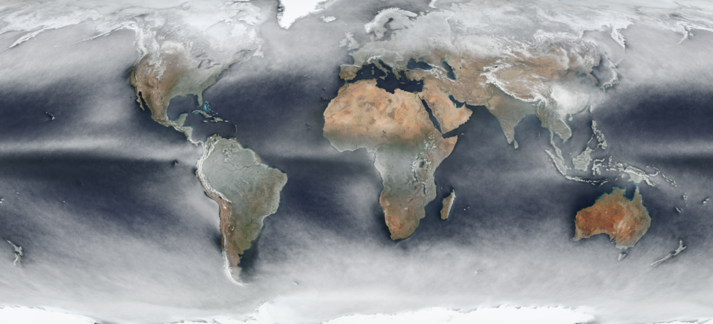
I collected all the daily images of the satellite-based Soumi VIIRS sensor and calculated the per-pixel average over the whole year of 2018.

You can explore it in full resolution in an interactive webmap.

WGS84 / Equirectangular
Web Mercator

You can see fascinating patterns, e.g. “downstream” of islands in the ocean or following big rivers like the Amazon. Be wary though as snow and clouds look the same here.

It’s also fun to look at the maximum to see cloudless regions (this image is highly exaggerated and does not make too much sense anyways):

Many thanks to Joshua Stevens for motivation and infos on data availability! The initial idea was of course inspired by Charlie ‘vruba’ Lyod‘s Cloudless atlas works. I explored imagery on https://worldview.earthdata.nasa.gov/, grabbed Soumi VIIRS images via https://wiki.earthdata.nasa.gov/display/GIBS/GIBS+API+for+Developers and processed it in GDAL. Poke me repeatedly to blog about the process please. (2022: Or don’t, I didn’t document it back then and can’t remember the final specifics. I think I did use imagemagick’s -evaluate-sequence median but might have done something in vips2 instead. The 2020 approach via GDAL is much easier.)

Full resolution, georeferenced imagery as Cloud-Optimized GeoTIFF:

*I said average but of course it is the median. The average or mean does not make much sense to use nor does it look any good. ;-)

zstandard compression in GeoTIFF

I ran GDAL 2.4’s gdal_translate (GDAL 2.4.0dev-333b907 or GDAL 2.4.0dev-b19fd35e6f-dirty, I am not sure) on some GeoTIFFs to compare the new ZSTD compression support to DEFLATE in file sizes and time taken.

Hardware was a mostly idle Intel(R) Xeon(R) CPU E3-1245 V2 @ 3.40GHz with fairly old ST33000650NS (Seagate Constellation) harddisks and lots of RAM.

A small input file was DGM1_2x2KM_XYZ_HH_2016-01-04.tif with about 40,000 x 40,000 pixels at around 700 Megabytes.
A big input file was srtmgl1.003.tif with about 1,3000,000 x 400,000 pixels at 87 Gigabytes.
Both input files had been DEFLATE compressed at the default level 6 without using a predictor (that’s what the default DEFLATE level will make them smaller here).

gdal_translate -co NUM_THREADS=ALL_CPUS -co PREDICTOR=2 -co TILED=YES -co BIGTIFF=YES --config GDAL_CACHEMAX 6144 was used all the time.
For DEFLATE -co COMPRESS=DEFLATE -co ZLEVEL=${level} was used, for ZSTD -co COMPRESS=ZSTD -co ZSTD_LEVEL=${level}

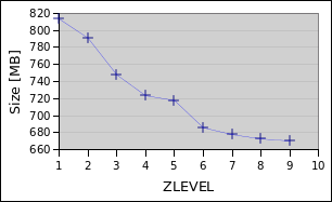
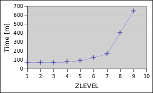
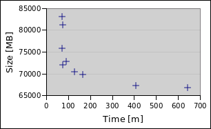
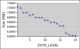
Mind the axes, sometimes I used a logarithmic scale!

Small file

DEFLATE

ZSTD

Big file

DEFLATE

ZSTD

Findings

It has been some weeks since I really looked at the numbers, so I am making the following up spontaneously. Please correct me!
Those numbers in the findings below should be percentages (between the algorithms, to their default values, etc), but my curiosity was satisfied. At the bottom is the data, maybe you can take it to present a nicer evaluation? ;)

ZSTD is powerful and weird. Sometimes subsequent levels might lead to the same result, sometimes a higher level will be fast or bigger. On low levels it is just as fast as DEFLATE or faster with similar or smaller sizes.

A <700 Megabyte version of the small file was accomplished within a minute with DEFLATE (6) or half a minute with ZSTD (5). With ZSTD (17) it got down to <600 Megabyte in ~5 Minutes, while DEFLATE never got anywhere near that.
Similarly for the big file, ZSTD (17) takes it down to 60 Gigabytes but it took almost 14 hours. DEFLATE capped at 65 Gigabytes. The sweet spot for ZSTD was at 10 with 4 hours for 65 Gigabytes (DEFLATE took 11 hours for that).

In the end, it is hard to say what default level ZSTD should take. For the small file level 5 was amazing, being even smaller than and almost twice as fast as the default (9). But for the big file the gains are much more gradual, here level 3 or level 10 stand out. I/O might be to blame?

Yes, the machine was not stressed and I did reproduce those weird ones.

Raw numbers

Small file

Algorithm Level Time [s] Size [Bytes] Size [MB] Comment
ZSTD 1 18 825420196 787
ZSTD 2 19 783437560 747
ZSTD 3 21 769517199 734
ZSTD 4 25 768127094 733
ZSTD 5 31 714610868 682
ZSTD 6 34 720153450 687
ZSTD 7 40 729787784 696
ZSTD 8 42 729787784 696
ZSTD 9 51 719396825 686 default
ZSTD 10 63 719394955 686
ZSTD 11 80 719383624 686
ZSTD 12 84 712429763 679
ZSTD 13 133 708790567 676
ZSTD 14 158 707088444 674
ZSTD 15 265 706788234 674
ZSTD 16 199 632481860 603
ZSTD 17 287 621778612 593
ZSTD 18 362 614424373 586
ZSTD 19 549 617071281 588
ZSTD 20 834 617071281 588
ZSTD 21 1422 616979884 588
DEFLATE 1 25 852656871 813
DEFLATE 2 26 829210959 791
DEFLATE 3 32 784069125 748
DEFLATE 4 31 758474345 723
DEFLATE 5 39 752578464 718
DEFLATE 6 62 719159371 686 default
DEFLATE 7 87 710755144 678
DEFLATE 8 200 705440096 673
DEFLATE 9 262 703038321 670

Big file

Algorithm Level Time [m] Size [Bytes] Size [MB] Comment
ZSTD 1 70 76132312441 72605
ZSTD 2 58 75351154492 71860
ZSTD 3 63 73369706659 69971
ZSTD 4 75 73343346296 69946
ZSTD 5 73 72032185603 68695
ZSTD 6 91 72564406429 69203
ZSTD 7 100 71138034760 67843
ZSTD 8 142 71175109524 67878
ZSTD 9 175 71175109524 67878 default
ZSTD 10 235 69999288435 66757
ZSTD 11 406 69999282203 66757
ZSTD 12 410 69123601926 65921
ZSTD 13 484 69123601926 65921
ZSTD 14 502 68477183815 65305
ZSTD 15 557 67494752082 64368
ZSTD 16 700 67494752082 64368
ZSTD 17 820 64255634015 61279
ZSTD 18 869 63595433364 60649
ZSTD 19 1224 63210562485 60282
ZSTD 20 2996 63140602703 60216
ZSTD 21 lolno
DEFLATE 1 73 87035905568 83004
DEFLATE 2 76 85131650648 81188
DEFLATE 3 73 79499430225 75817
DEFLATE 4 77 75413492394 71920
DEFLATE 5 92 76248511117 72716
DEFLATE 6 129 73901542836 70478 default
DEFLATE 7 166 73120114047 69733
DEFLATE 8 407 70446588490 67183
DEFLATE 9 643 70012677124 66769

Specifying the read/open driver/format with GDAL/OGR

For the commandline utilities you can’t. One possible workaround is using https://trac.osgeo.org/gdal/wiki/ConfigOptions#GDAL_SKIP and https://trac.osgeo.org/gdal/wiki/ConfigOptions#OGR_SKIP to blacklist drivers until the one you want is its first choice. A feature request exists at https://trac.osgeo.org/gdal/ticket/5917 but it seems that the option is not exposed as commandline option (yet?).

PS: If what you are trying to do is reading a .txt (or whatever) file as .csv and you get angry at the CSV driver only being selected if the file has a .csv extension, use CSV:yourfilename.txt

PPS: This post was motivated by not finding above information when searching the web. Hopefully this will rank high enough for *me* to find it next time. ;)

One SRTMGL1 GeoTIFF to rule them all

NOTE: In up to date GDAL things might be easier AND I messed up with --config and -co below. Poke me to update it please.

So about half a year ago Lukas Martinelli asked about a global SRTM GeoTIFF. The SRTM elevation data is usually shared in many small tiles which can be ideal for some cases but annoying for others. I like downloading and processing big files so I took that as a challenge. It’s probably some mental thing. I never finished this blog post back then. It’s probably another mental thing. 8) Read on if you are interested in some GNU coreutils hackery as well as GDAL magick.

Here is how I did it. Endless thanks as usual to Even Rouault who fixed GDAL bugs and gave great hints. I learned more about GeoTIFFs and GDAL than I should have needed to know.

Downloading the source files

The source files are available at http://e4ftl01.cr.usgs.gov/SRTM/SRTMGL1.003/2000.02.11/ (warning, visiting this URL will make your browser cry and potentially render your system unresponsive). To download them you must create an NASA Earthdata Login at https://urs.earthdata.nasa.gov/users/new/. :\

********************************************************************************

                         U.S. GOVERNMENT COMPUTER

This US Government computer is for authorized users only.  By accessing this
system you are consenting to complete monitoring with no expectation of privacy.
Unauthorized access or use may subject you to disciplinary action and criminal
prosecution.

OMGOMGOMG. I am sure they would have used <blink> if accessibility guidelines allowed it. As I am not sure what their Terms of Service are, I will not give you a copy’n’paste ready line to download them all. wget or aria2 work well. You should get 14297 files with a total size of 98G.

Inspecting the ZIP files and preparing for GDAL’s vsizip

Each of those ZIP files has just a single file “.hgt” inside. GDAL specifically has support for the “SRTM HGT Format“, so we know it can read those files. We just need to extract them. (If you clicked that link you see that with GDAL 2.2 it will support directly loading the data from the ZIPs, that’s just Even being awesome.)

We don’t want to uncompress all those files just because we want to build a GeoTIFF from them later, do we? Luckily GDAL has a vsizip thingie which allows it to read files inside zip archives. Wicked! For this we need the “deep” paths to the files though, for example e4ftl01.cr.usgs.gov/SRTM/SRTMGL1.003/2000.02.11/N29E000.SRTMGL1.hgt.zip/N29E000.hgt.

The files inside the archives are always simply the same filename minus the “.SRTMGL1” and the .zip extension. Perfect, now we know all the files from inside the ZIPs! Right? Nope. Unfortunately some (17) of the archives do include the “.SRTMGL1” bit in their files, for example N38E051.SRTMGL1.hgt… >:(

That’s why we need to look into each zip file and determine the filename inside. (Alternatively *you* could extract them all after all, you with your fancy, huge SSD.)

We can simply use `unzip` with the `-t` switch to make it show what’s inside (and as a “free” benefit it will also check the file’s integrity for us). `tee` is used here to save the output to a file. This will take a while as it needs to read through all the files…

$ unzip -t "e4ftl01.cr.usgs.gov/SRTM/SRTMGL1.003/2000.02.11/*.SRTMGL1.hgt.zip" | tee unzip-t.log

...

Archive: e4ftl01.cr.usgs.gov/SRTM/SRTMGL1.003/2000.02.11/N29E000.SRTMGL1.hgt.zip
testing: N29E000.hgt OK
No errors detected in compressed data of e4ftl01.cr.usgs.gov/SRTM/SRTMGL1.003/2000.02.11/N29E000.SRTMGL1.hgt.zip.

Archive: e4ftl01.cr.usgs.gov/SRTM/SRTMGL1.003/2000.02.11/N27E033.SRTMGL1.hgt.zip
testing: N27E033.hgt OK
No errors detected in compressed data of e4ftl01.cr.usgs.gov/SRTM/SRTMGL1.003/2000.02.11/N27E033.SRTMGL1.hgt.zip.

Archive: e4ftl01.cr.usgs.gov/SRTM/SRTMGL1.003/2000.02.11/N45E066.SRTMGL1.hgt.zip
testing: N45E066.hgt OK
No errors detected in compressed data of e4ftl01.cr.usgs.gov/SRTM/SRTMGL1.003/2000.02.11/N45E066.SRTMGL1.hgt.zip.

14297 archives were successfully processed.

Yay, no errors!

In the output we see the path to the archive and we see the name of the file inside. With some sed and grep we can easily construct “deep” paths.

First we remove the status lines, the blank lines and the very last full status line with `grep`:

$ cat unzip-t.log | grep -v -e "No errors" -e '^$' -e 'successfully processed'

Archive: e4ftl01.cr.usgs.gov/SRTM/SRTMGL1.003/2000.02.11/N12E044.SRTMGL1.hgt.zip
testing: N12E044.hgt OK
Archive: e4ftl01.cr.usgs.gov/SRTM/SRTMGL1.003/2000.02.11/N29W002.SRTMGL1.hgt.zip
testing: N29W002.hgt OK
Archive: e4ftl01.cr.usgs.gov/SRTM/SRTMGL1.003/2000.02.11/N45E116.SRTMGL1.hgt.zip
testing: N45E116.hgt OK

Then we concatenate every consecutive two lines into one line with `paste` (I LOVE THIS 1 TRICK!):

$ cat unzip-t.log | grep -v -e "No errors" -e '^$' -e 'successfully processed' | paste - -

Archive: e4ftl01.cr.usgs.gov/SRTM/SRTMGL1.003/2000.02.11/N12E044.SRTMGL1.hgt.zip testing: N12E044.hgt OK
Archive: e4ftl01.cr.usgs.gov/SRTM/SRTMGL1.003/2000.02.11/N29W002.SRTMGL1.hgt.zip testing: N29W002.hgt OK
Archive: e4ftl01.cr.usgs.gov/SRTM/SRTMGL1.003/2000.02.11/N45E116.SRTMGL1.hgt.zip testing: N45E116.hgt OK

Finally we strip things away with sed (I don’t care that you would do it differently, this is how I quickly did it with my flair of hammering) and direct the output into a new file called `zips`:

$ cat unzip-t.log | grep -v -e "No errors" -e '^$' -e 'successfully processed' | paste - - | sed -e 's#Archive:[ ]*##' -e 's#\t[ ]*testing: #/#' -e 's#[ ]*OK##' > zips

e4ftl01.cr.usgs.gov/SRTM/SRTMGL1.003/2000.02.11/N12E044.SRTMGL1.hgt.zip/N12E044.hgt
e4ftl01.cr.usgs.gov/SRTM/SRTMGL1.003/2000.02.11/N29W002.SRTMGL1.hgt.zip/N29W002.hgt
e4ftl01.cr.usgs.gov/SRTM/SRTMGL1.003/2000.02.11/N45E116.SRTMGL1.hgt.zip/N45E116.hgt

Yay, we have all the actual inside-zip paths now!

If you are curious, you can try gdalinfo with those now. You need to prepend /vsizip/ to the path to make it read inside zip files.

$ gdalinfo /vsizip/e4ftl01.cr.usgs.gov/SRTM/SRTMGL1.003/2000.02.11/N12E044.SRTMGL1.hgt.zip/N12E044.hgt

Driver: SRTMHGT/SRTMHGT File Format
Files: /vsizip/e4ftl01.cr.usgs.gov/SRTM/SRTMGL1.003/2000.02.11/N12E044.SRTMGL1.hgt.zip/N12E044.hgt
Size is 3601, 3601
Coordinate System is:
GEOGCS["WGS 84",
    DATUM["WGS_1984",
        SPHEROID["WGS 84",6378137,298.257223563,
            AUTHORITY["EPSG","7030"]],
        AUTHORITY["EPSG","6326"]],
    PRIMEM["Greenwich",0,
        AUTHORITY["EPSG","8901"]],
    UNIT["degree",0.0174532925199433,
        AUTHORITY["EPSG","9122"]],
    AUTHORITY["EPSG","4326"]]
Origin = (43.999861111111109,13.000138888888889)
Pixel Size = (0.000277777777778,-0.000277777777778)
Metadata:
  AREA_OR_POINT=Point
Corner Coordinates:
Upper Left  (  43.9998611,  13.0001389) ( 43d59'59.50"E, 13d 0' 0.50"N)
Lower Left  (  43.9998611,  11.9998611) ( 43d59'59.50"E, 11d59'59.50"N)
Upper Right (  45.0001389,  13.0001389) ( 45d 0' 0.50"E, 13d 0' 0.50"N)
Lower Right (  45.0001389,  11.9998611) ( 45d 0' 0.50"E, 11d59'59.50"N)
Center      (  44.5000000,  12.5000000) ( 44d30' 0.00"E, 12d30' 0.00"N)
Band 1 Block=3601x1 Type=Int16, ColorInterp=Undefined
  NoData Value=-32768
  Unit Type: m

Hooray! GDAL reads the hgt file from inside its zip!

We need to prepend all the paths with `/vsizip/` so let’s do that:

$ sed 's#^#/vsizip/##' zips > vsizips

/vsizip/e4ftl01.cr.usgs.gov/SRTM/SRTMGL1.003/2000.02.11/N12E044.SRTMGL1.hgt.zip/N12E044.hgt
/vsizip/e4ftl01.cr.usgs.gov/SRTM/SRTMGL1.003/2000.02.11/N29W002.SRTMGL1.hgt.zip/N29W002.hgt
/vsizip/e4ftl01.cr.usgs.gov/SRTM/SRTMGL1.003/2000.02.11/N45E116.SRTMGL1.hgt.zip/N45E116.hgt

Unfortunately those 17 misnamed files from earlier need special treatment… This is what my notes say, not sure what it was supposed to do. If you are recreating this all, please just ask me and I will look at it again. For now, let’s just pretend that this leads to a file called `hgtfiles` in which all the paths are perfect and all the files are perfect.


grep -v 'SRTMGL1.hgt$' vsizips > vsizipswithoutmisnamedfiles
mkdir misnamedfiles
cd misnamedfiles/
nano ../listofmisnamedfiles # insert the paths to those 17 zips here #TODO
while read filename; do unzip "../${filename}"; done < ../listofmisnamedfiles
rename 's/SRTMGL1.//' *.hgt
cd ..
find misnamedfiles/ -type f > listofmisnamedfileshgt
cat listofmisnamedfileshgt vsizipswithoutmisnamedfiles > hgtfiles

As I said above though, go with a recent GDAL and this is all much easier. Even even included a check for the different filenames inside, how can you not like that guy!

Building a Virtual Raster Table

Virtual Raster Tables (VRT) are some kind of files that pretend to be rasters. They are awesome. Here we use a VRT that simply turns all the small rasters we have into one big ass raster.

Ok, ready to create a Virtual Raster Table!

$ time gdalbuildvrt -input_file_list hgtfiles srtmgl1.003.vrt

0...10...20...30...40...50...60...70...80...90...100 - done.

real 0m22.679s
user 0m19.250s
sys 0m3.105s

Done.

You could go ahead and use this for your work/leisure now. But remember, it is tens of gigabytes of data so if you do not use it at a 1:1 scale things will not be fun and might fry your cat. You want overviews/pyramids.

Turning the VRT into a GeoTIFF (Optional)

Let’s make a HUGEGEOTIFF because that’s cool! You don’t have to, instead you could build overviews for the .vrt file.

We want it quick to read and small so I used DEFLATE, TILED and the horizontal predictor. I ran this on a weak i7 with 2G of RAM and can’t remember what the worst bottleneck was. Probably CPU.

$ time gdal_translate -co NUM_THREADS=ALL_CPUS --config PREDICTOR 2 -co COMPRESS=DEFLATE -co TILED=YES -co BIGTIFF=YES srtmgl1.003.vrt srtmgl1.003.vrt.tif

Input file size is 1296001, 417601
0...10...20...30...40...50...60...70...80...90...100 - done.

real 231m57.961s
user 503m23.044s
sys 3m14.600s

If you are courageous you can load that file in your GIS now. But again, unless you watch it at a 1:1 scale or something close to that it WILL not be much fun and potentially expose weaknesses in your GIS and fill up your system’s memory and crash and you had no unsaved work open, didn’t you?

Building Overviews

Overviews aka pyramids are usually about 1/3 the size of the full image. If they are not, you probably used different compression settings. This was the step that I expected to be just boring to wait for, but it turned out the most problematic. I tried all available free tools but none worked properly with an input this big. With GDAL we found a workaround after a while.

gdaladdo has problems building multiple overview levels with a file this big… The trick is to built the overviews sequentially, not in one invocation. The best solution at the moment was building overviews for overviews for overviews and so on until you reach a comfortable size. Something like:


gdaladdo -ro srtmgl1.003.tif 2
gdaladdo -ro srtmgl1.003.tif.ovr 2
gdaladdo -ro srtmgl1.003.tif.ovr.ovr 2
gdaladdo -ro srtmgl1.003.tif.ovr.ovr.ovr 2
gdaladdo -ro srtmgl1.003.tif.ovr.ovr.ovr.ovr 2 4 8 16 32 64 128 256 512

I used the following parameters:
gdaladdo -oo NUM_THREADS=ALL_CPUS --config GDAL_NUM_THREADS ALL_CPUS --config GDAL_CACHEMAX 2048 --config COMPRESS_OVERVIEW DEFLATE --config PREDICTOR_OVERVIEW 2 --config BIGTIFF_OVERVIEW YES -ro

ovrovrovrovrovrovrovrovrovrovr

Apparently gdaladdo automatically makes them tiled, which is good. I used https://gist.github.com/springmeyer/3007985 to find out.

Creating overviews took just about 3 hours with this weird trick. So, in total the processing just takes half a day.

Download

Enjoy! https://www.datenatlas.de/geodata/public/srtmgl1/. I impose no license/copyright/whatever on this derivative work.

TODO

Hillshading? Slope? You do it!

Found a better, faster way? You blog it!

We could add the overviews to the main image with `gdal_translate srtmgl1.003.tif srtmgl1.003.withovr.tif -co COPY_SRC_OVERVIEWS=YES [other options]` says Even.
Fancy Free File Formats For Hamburg’s Open Geodata

While this is about data of the city of Hamburg, Germany, I decided to post in English as GeoPackage Propaganda should be accessible. ;)
I am casually working on converting open geodata released via the Transparenzportal Hamburg to more usable GeoPackages, GeoTIFFs and similar formats with free and open-source tools like GDAL and GMT where possible. This includes things like orthophotos, ALKIS, addresses, DEM, districts etc. You can get a list of most available source data here but there are some datasets “hidden” in other categories as well. The data is usually released in GML or as gridded files (e.g. JPEG or XYZ tiles/files). While this is pretty much perfect as source formats, working with them is cumbersome. My goal is to make this data more accessible for anyone in tools like QGIS.

For now you can find the 20cm orthophotos for 2013-2015 and the 1m DEM in https://www.datenatlas.de/geodata/public/hamburg/. Mind the licenses, see the readme file for a bit of info. More to come, I want to plan the pipeline a bit better first though. There should be a full script & log from source to GeoPackage for each file.

I will also provide mirrors of the source files. If you want to collaborate, please contact me. Apart from Hamburg I will also add free/open datasets for the whole of Germany, things related to (nearby) bathymetry and some global ones. If you want Shapefiles, ECW, MrSID or similar, you can pay me for converting.

Merge GML files into one SQLite or Spatialite file

For example the buildings in Hamburg, Germany:

layer=$1
for file in *.xml
do
 if [ -f "${layer}".spatialite ]
 then
  ogr2ogr -f "SQLite" -update -append "${layer}".spatialite "${file}" "${layer}" -dsco SPATIALITE=YES
 else
  ogr2ogr -a_srs EPSG:25832 -f "SQLite" "${layer}".spatialite "${file}" "${layer}" -dsco SPATIALITE=YES
 fi
done

Remove the -dsco SPATIALITE=YES and change the output filename for SQLite. QGIS can work with both.

$ bash mergexmltospatialite.sh AX_Gebaeude

Be aware that Spatialite is much more sensitive to geometric problems. You might get things like

ERROR 1: sqlite3_step() failed:
ax_gebaeude.GEOMETRY violates Geometry constraint [geom-type or SRID not allowed] (19)
ERROR 1: ROLLBACK transaction failed: cannot rollback - no transaction is active
ERROR 1: Unable to write feature 1712 from layer AX_Gebaeude.

ERROR 1: Terminating translation prematurely after failed translation of layer AX_Gebaeude (use -skipfailures to skip errors)

but on the other hand, you get spatial indexing which makes queries or high zoom interaction much quicker.

Be aware that if you try to merge files into a Shapefile and fields are getting truncated, those fields will only be filled with data for the first file you merge. On the later files OGR will try to match the input field names to the merged file’s fieldnames, notice the difference and discard them. If you still want to convert to Shapefiles, check out the -fieldTypeToString IntegerList,StringList options.