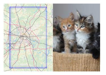
Recorded by placing two windows side by side and zoom into separate, non-cached regions using:"xte "mousemove 640 440" "mouseclick 4" && xte "mousemove 1080 440" "mouseclick 4" in a loop.
Category Archives: GIS
Von wo wurde der Hamburger Fernsehturm fotografiert
Vom großartigen @Fernsehturm_HH-Account inspiriert hab ich mal ein 4 Jahre altes Projektchen aufgewärmt: Verortete Fotos auf Flickr, die mit “Hamburg” und “Fernsehturm” getaggt sind. Alternativ als Linien vom (angeblichen) Aufnahmeort zum Turm.
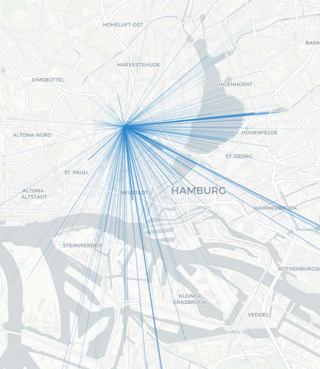
Ungefiltert und voller Mist, aber man kann z. B. toll sehen, wie einladend die Brückem vorm Kuhmühlenteich für Fotos sind.
Kostenlose Internetpunkteabsahnidee: Dasselbe mit dem Eiffelturm, dem Londoner Dildo u. ä. machen, Konkave Hülle außen drum, schick aufbereiten, als “Nur wo man $Wahrzeichen sieht, ist $Stadt” vermarkten, €€€€.
Interaktive Karte der Baugenehmigungen in Hamburg
Ich habe endlich mal ein über mehrere Jahre gereiftes (eher gealtertes und verfrickeltes) Projekt in einen einigermaßen vorzeigbaren Zustand gebracht: Eine interaktive Karte der Baugenehmigungen in Hamburg.
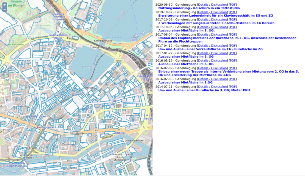
Je weniger transparent eine Fläche dargestellt ist, desto mehr Dokumente sind mit ihr verknüpft (ja, es ist ein Feature je Dokument D;). Eigentlich war die Seite anders aufgebaut, mit einem PDF-Viewer auf der rechten Seite. Aber da daten.transparenz.hamburg.de kein HTTPS kann (seid ihr auch so gespannt auf die UMTS-Auktion nächste Woche?), geht das aus Sicherheitsgründen nicht ohne ein Spiegeln der Daten oder einen Proxy.
Die Daten kommen größtenteils aus dem Transparenzportal. Für das Matching der angebenen Flurstücks-“IDs” zu den tatsächlichen Flurstücken war aber ein erheblicher Aufwand nötig. Das Drama ging bis hin zum Parsen aus PDFs, die mal so, mal so formatiert waren und natürlich auch voller Eingabefehler auf Behördenseite. Vielleicht schreibe ich da noch beizeiten mal einen Rant. TL;DR: Ohne die zugehörige Gemarkung ist mit einer Flurstücks-“ID” wie in den Daten angegeben keine räumliche Zuordnung möglich. In den veröffentlichten Daten stecken nur die Nenner der Flurstücksnummern, nicht aber die Gemarkungsnummern. Ziemlich absurd.
Das ganze ist nur ein Prototyp, vermutlich voller Fehler und fehlender Daten. Aber interessant und spaßig ist es, viel Freude also!
Es wäre noch eine MENGE zu tun, um das ganze rund zu machen. Falls du Lust hast, melde dich gerne. Es geht vom wilden Parsen, über Sonderregeln für kaputte Dokumente, zu Kartenstyling bis zur UI. Schön wäre es auch alles in einer anständigen Datenbank zu halten und nicht nur nach der räumlichen Dimension durchsuchen zu können.
Highlight current timeslice in a QGIS Atlas layout
Did this for an ex-colleague some months ago and forgot to share the how-to publically. We needed a visual representation of the current time in a layout that showed both a raster map (different layer per timeslice) and a timeseries plot of an aspect of the data (this was created outside QGIS).
Have lots of raster layers you want to iterate through. I have:
./ECMWF_ERA_40_subset/2019-01-01.tif
./ECMWF_ERA_40_subset/2019-01-02.tif
./ECMWF_ERA_40_subset/2019-01-03.tif
./ECMWF_ERA_40_subset/2019-01-04.tif
./ECMWF_ERA_40_subset/2019-01-05.tif
./ECMWF_ERA_40_subset/2019-01-06.tif
...
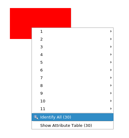
Create a new layer for your map extent. Draw your extent as geometry. Duplicate that geometry as many times as you have days. Alternatively you could of course have different geometries per day. Whatever you do, you need a layer with one feature per timeslice for the Atlas to iterate though. I have 30 days to visualise so I duplicated my extent 30 times.
Open the Field Calculator. Add a new field called date as string type (not as date type until some bug is fixed (sorry, did not make a note here, maybe sorting is/was broken?)) with an expression that represents time and orders chronologically if sorted by QGIS. For example: '2019-01-' || lpad(@row_number,2,0) (assuming your records are in the correct order if you have different geometries…)
Have your raster layers named the same way as the date attribute values.
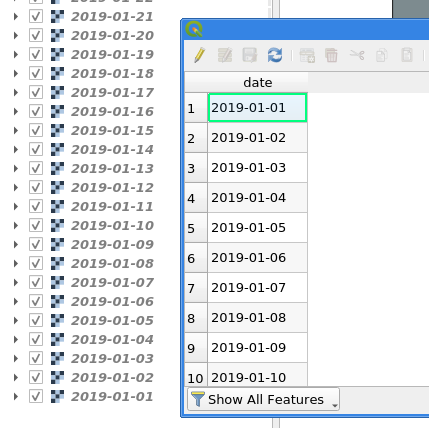
Make a new layout.
For your Layout map check “Lock layers” and use date as expression for the “Lock layers” override. This will now select the appropriate raster layer, based on the attribute value <-> layer name, to display for each Atlas page.
Cool, if you preview the Atlas now you got a nice animation through your raster layers. Let’s do part 2:
In your layout add your timeseries graph. Give it a unique ID, e. g. “plot box”. Set its width and height via new variables (until you can get those via an expression this is needed for calculations below).
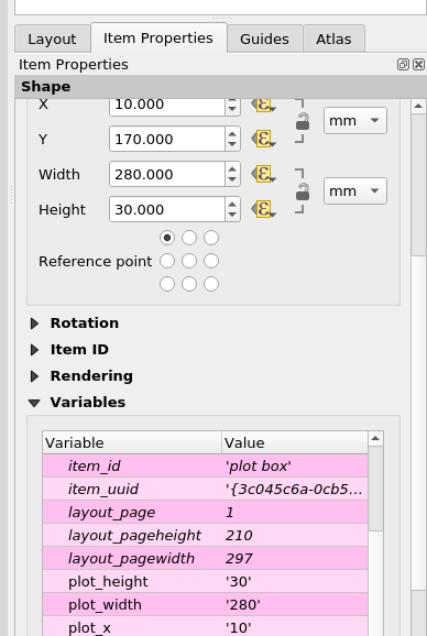
Create a box to visualise the timeslice. Set its width to map_get(item_variables('plot box'), 'plot_width') / @atlas_totalfeatures. For the height and y use/adjust this expression: map_get(item_variables('plot box'), 'plot_height'). For x comes the magic:
with_variable(
     'days_total',
     day(to_date(maximum("date"))-to_date(minimum("date")))+1,
       -- number of days in timespan
       -- +1 because we need the number of days in total
       -- not the inbetween, day() to just get the number of days
     with_variable(
         'mm_per_day',
         map_get(item_variables('plot box'), 'plot_width') / @days_total,
         with_variable(
             'days',
             day(to_date(attribute(@atlas_feature, 'date'))-to_date(minimum("date"))),
               -- number of days the current feature is from the first day
               -- to_date because BUG attribute() returns datetime for date field
             @mm_per_day * @days + map_get(item_variables('plot box'), 'plot_x')
         )
     )
 )
This will move the box along the x axis accordingly.
Have fun!
How to get a dataset out of OpenStreetMap (OSM) and into QGIS easily
For small datasets just use the QuickOSM plugin, enter your key=value and it will load the data directly as QGIS layer(s).
For big datasets don’t run massive queries on the Overpass API but use prepared thematic or regional OpenStreetMap extracts.
For example, if you want all things tagged place=town globally, grab place_EPSG4326.zip from http://download.osmdata.xyz/ and run a filter on that locally.
Don’t be scared of processing a global OSM planet file either, Osmium makes filtering OSM data extremely easy:
osmium tags-filter in.osm.pbf n/place=town -o place=town.osm.pbf
Yes, a planet file is pretty big, but extracting specific features from that is not a big data problem and you must not be scared of it. Downloading the file will probably take you magnitudes longer than extracting something from it. For me it was 45 minutes for the download, then about 8 minutes for extracting on a seriously slow (~60MB/s) spinning metal hard disk drive (no SSD).
And yes, you can load OSM PBF directly into QGIS thanks to GDAL’s support for the format.
While we are at it: Don’t use GeoJSON for anything but data transfer and maybe storage. It is not an efficient format to power your layers and GIS analyses. (OSM PDF isn’t either.)
Make sure you actually do use spatial indexes
Ever ran some GIS analysis in QGIS and it took longer than a second? Chances are that your data did not have spatial indexes for QGIS to utilise and that it could have been magnitudes faster.
I realised just today, after years of using QGIS, that it did not automatically create a spatial index when saving a Shapefile. And because of that, lots of GIS stuff I did in the past, involving saving subsets of data to quick’n’dirty Shapefiles, was slower than necessary.
Sadly QGIS does not communicate lack of spatial indexing to the user in any way. I added a feature request to make Processing warn if no indexing is available.
An example: Running ‘Count points in polygon’ on 104 polygons with 223210 points:
- Points in original GML file: 449 seconds
- GML is not a format for processing but meant for data transfer, never ever think of using it for anything else
- Points in ESRI Shapefile: 30 seconds
- Points in GeoPackage: 3 seconds
- Points in ESRI Shapefile with spatial index: 3 seconds
- Same Shapefile as before but this time I had created a .qix index

So yeah, make sure you don’t only use a reasonable format for your data. And also make sure you do actually have an spatial index.
For Shapefiles, look for a .qix or .sbn side-car file somewhere in the heap of files. In QGIS you can create a spatial index for a vector layer either using the “Create spatial index” algorithm in Processing or the button of the same title in the layer properties’ source tab.
PS: GeoPackages always have a spatial index. That’s reason #143 why they are awesome.
Calculating the metric distance between latitudes with PostGIS
Postgres’ WITH clauses and window functions are so awesome.
-- generate values from -90 to 90, increment by 1
WITH values AS (
  SELECT generate_series AS latitude
  FROM generate_series(-90, 90)
),
-- create a geographic point each
points AS (
  SELECT ST_MakePoint(0, latitude)::geography AS point FROM values
)
SELECT
  -- latitude values of subsequent points
  format(
    '%s° to %s°',
    ST_Y(point::geometry),
    ST_Y(lag(point::geometry) OVER ())
  ) AS latitudes,
  -- geographic distance between subsequent points, formatted to kilometers
  format(
    '%s km',
    to_char(ST_Distance(point, lag(point) OVER ())/1000, '999D99')
  ) AS distance
FROM points
OFFSET 1  -- skip the first row, no lag there
;

    latitudes  |  distance
 --------------+------------
  -89° to -90° |  111.69 km
  -88° to -89° |  111.69 km
  -87° to -88° |  111.69 km
  -86° to -87° |  111.69 km
  -85° to -86° |  111.69 km
  -84° to -85° |  111.68 km
  -83° to -84° |  111.68 km
  -82° to -83° |  111.67 km
  -81° to -82° |  111.67 km
  -80° to -81° |  111.66 km
  -79° to -80° |  111.66 km
  -78° to -79° |  111.65 km
  -77° to -78° |  111.64 km
  -76° to -77° |  111.63 km
  -75° to -76° |  111.62 km
  -74° to -75° |  111.61 km
  -73° to -74° |  111.60 km
  -72° to -73° |  111.59 km
  -71° to -72° |  111.58 km
  -70° to -71° |  111.57 km
  -69° to -70° |  111.56 km
  -68° to -69° |  111.54 km
  -67° to -68° |  111.53 km
  -66° to -67° |  111.51 km
  -65° to -66° |  111.50 km
  -64° to -65° |  111.49 km
  -63° to -64° |  111.47 km
  -62° to -63° |  111.45 km
  -61° to -62° |  111.44 km
  -60° to -61° |  111.42 km
  -59° to -60° |  111.40 km
  -58° to -59° |  111.39 km
  -57° to -58° |  111.37 km
  -56° to -57° |  111.35 km
  -55° to -56° |  111.33 km
  -54° to -55° |  111.31 km
  -53° to -54° |  111.30 km
  -52° to -53° |  111.28 km
  -51° to -52° |  111.26 km
  -50° to -51° |  111.24 km
  -49° to -50° |  111.22 km
  -48° to -49° |  111.20 km
  -47° to -48° |  111.18 km
  -46° to -47° |  111.16 km
  -45° to -46° |  111.14 km
  -44° to -45° |  111.12 km
  -43° to -44° |  111.10 km
  -42° to -43° |  111.08 km
  -41° to -42° |  111.06 km
  -40° to -41° |  111.04 km
  -39° to -40° |  111.03 km
  -38° to -39° |  111.01 km
  -37° to -38° |  110.99 km
  -36° to -37° |  110.97 km
  -35° to -36° |  110.95 km
  -34° to -35° |  110.93 km
  -33° to -34° |  110.91 km
  -32° to -33° |  110.90 km
  -31° to -32° |  110.88 km
  -30° to -31° |  110.86 km
  -29° to -30° |  110.84 km
  -28° to -29° |  110.83 km
  -27° to -28° |  110.81 km
  -26° to -27° |  110.80 km
  -25° to -26° |  110.78 km
  -24° to -25° |  110.77 km
  -23° to -24° |  110.75 km
  -22° to -23° |  110.74 km
  -21° to -22° |  110.72 km
  -20° to -21° |  110.71 km
  -19° to -20° |  110.70 km
  -18° to -19° |  110.69 km
  -17° to -18° |  110.67 km
  -16° to -17° |  110.66 km
  -15° to -16° |  110.65 km
  -14° to -15° |  110.64 km
  -13° to -14° |  110.63 km
  -12° to -13° |  110.63 km
  -11° to -12° |  110.62 km
  -10° to -11° |  110.61 km
  -9° to -10°  |  110.60 km
  -8° to -9°   |  110.60 km
  -7° to -8°   |  110.59 km
  -6° to -7°   |  110.59 km
  -5° to -6°   |  110.58 km
  -4° to -5°   |  110.58 km
  -3° to -4°   |  110.58 km
  -2° to -3°   |  110.58 km
  -1° to -2°   |  110.58 km
  0° to -1°    |  110.57 km
  1° to 0°     |  110.57 km
  2° to 1°     |  110.58 km
  3° to 2°     |  110.58 km
  4° to 3°     |  110.58 km
  5° to 4°     |  110.58 km
  6° to 5°     |  110.58 km
  7° to 6°     |  110.59 km
  8° to 7°     |  110.59 km
  9° to 8°     |  110.60 km
  10° to 9°    |  110.60 km
  11° to 10°   |  110.61 km
  12° to 11°   |  110.62 km
  13° to 12°   |  110.63 km
  14° to 13°   |  110.63 km
  15° to 14°   |  110.64 km
  16° to 15°   |  110.65 km
  17° to 16°   |  110.66 km
  18° to 17°   |  110.67 km
  19° to 18°   |  110.69 km
  20° to 19°   |  110.70 km
  21° to 20°   |  110.71 km
  22° to 21°   |  110.72 km
  23° to 22°   |  110.74 km
  24° to 23°   |  110.75 km
  25° to 24°   |  110.77 km
  26° to 25°   |  110.78 km
  27° to 26°   |  110.80 km
  28° to 27°   |  110.81 km
  29° to 28°   |  110.83 km
  30° to 29°   |  110.84 km
  31° to 30°   |  110.86 km
  32° to 31°   |  110.88 km
  33° to 32°   |  110.90 km
  34° to 33°   |  110.91 km
  35° to 34°   |  110.93 km
  36° to 35°   |  110.95 km
  37° to 36°   |  110.97 km
  38° to 37°   |  110.99 km
  39° to 38°   |  111.01 km
  40° to 39°   |  111.03 km
  41° to 40°   |  111.04 km
  42° to 41°   |  111.06 km
  43° to 42°   |  111.08 km
  44° to 43°   |  111.10 km
  45° to 44°   |  111.12 km
  46° to 45°   |  111.14 km
  47° to 46°   |  111.16 km
  48° to 47°   |  111.18 km
  49° to 48°   |  111.20 km
  50° to 49°   |  111.22 km
  51° to 50°   |  111.24 km
  52° to 51°   |  111.26 km
  53° to 52°   |  111.28 km
  54° to 53°   |  111.30 km
  55° to 54°   |  111.31 km
  56° to 55°   |  111.33 km
  57° to 56°   |  111.35 km
  58° to 57°   |  111.37 km
  59° to 58°   |  111.39 km
  60° to 59°   |  111.40 km
  61° to 60°   |  111.42 km
  62° to 61°   |  111.44 km
  63° to 62°   |  111.45 km
  64° to 63°   |  111.47 km
  65° to 64°   |  111.49 km
  66° to 65°   |  111.50 km
  67° to 66°   |  111.51 km
  68° to 67°   |  111.53 km
  69° to 68°   |  111.54 km
  70° to 69°   |  111.56 km
  71° to 70°   |  111.57 km
  72° to 71°   |  111.58 km
  73° to 72°   |  111.59 km
  74° to 73°   |  111.60 km
  75° to 74°   |  111.61 km
  76° to 75°   |  111.62 km
  77° to 76°   |  111.63 km
  78° to 77°   |  111.64 km
  79° to 78°   |  111.65 km
  80° to 79°   |  111.66 km
  81° to 80°   |  111.66 km
  82° to 81°   |  111.67 km
  83° to 82°   |  111.67 km
  84° to 83°   |  111.68 km
  85° to 84°   |  111.68 km
  86° to 85°   |  111.69 km
  87° to 86°   |  111.69 km
  88° to 87°   |  111.69 km
  89° to 88°   |  111.69 km
90° to 89° | 111.69 kmOpen Layers View Tracker
I built this last year for some research and then swiftly forgot about releasing it to the public. Here it is now:
https://gitlab.com/Hannes42/OpenLayersViewTracker
Try it online: https://hannes42.gitlab.io/OpenLayersViewTracker/
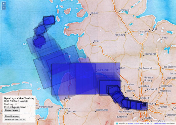
Some awful but working JavaScript code to track a website user’s interaction with a Open Layers map. You can use this to do awesome user studies and experiments.
- Runs client-side
- You will get a polygon of each “view”!
- You can look at them in the browser!
- There are also timestamps! Hyperaccurate in milliseconds since unix epoch!
- And a GeoJSON export!
- This works with rotated views!
- Written for Open Layers 4 using some version of JSTS, see the libs/ directory. No idea if it works with the latest versions or if Open Layers changed their API again.
Please do some funky research with it and tell me about your experiences! Apart from that, you are on your own.
There is a QGIS project with example data included. Check out the Atlas setup in the Print Layout!
Screenshot from a browser session
Resulting GeoJSON in QGIS
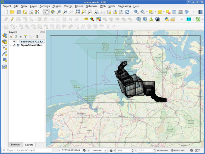
So if Time Manager supports the timestamp format you could interactively scroll around. I did not try, that plugin is so finicky.
Average Earth from Space 2018
I collected all the daily images of the satellite-based Soumi VIIRS sensor and calculated the per-pixel average over the whole year of 2018.
You can explore it in full resolution in an interactive webmap.

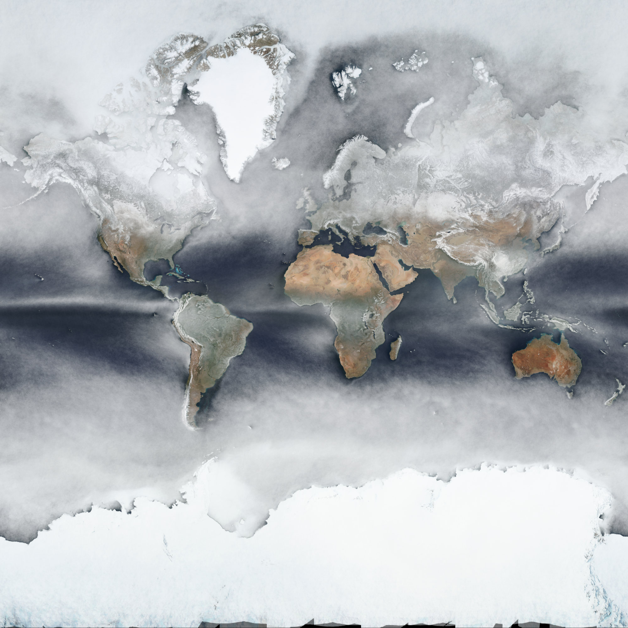
You can see fascinating patterns, e.g. “downstream” of islands in the ocean or following big rivers like the Amazon. Be wary though as snow and clouds look the same here.
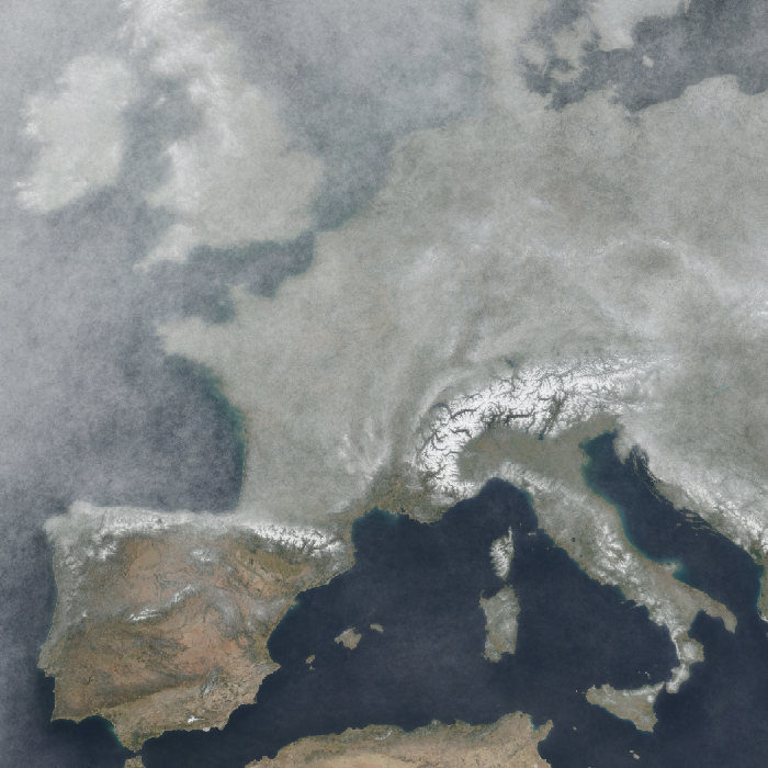


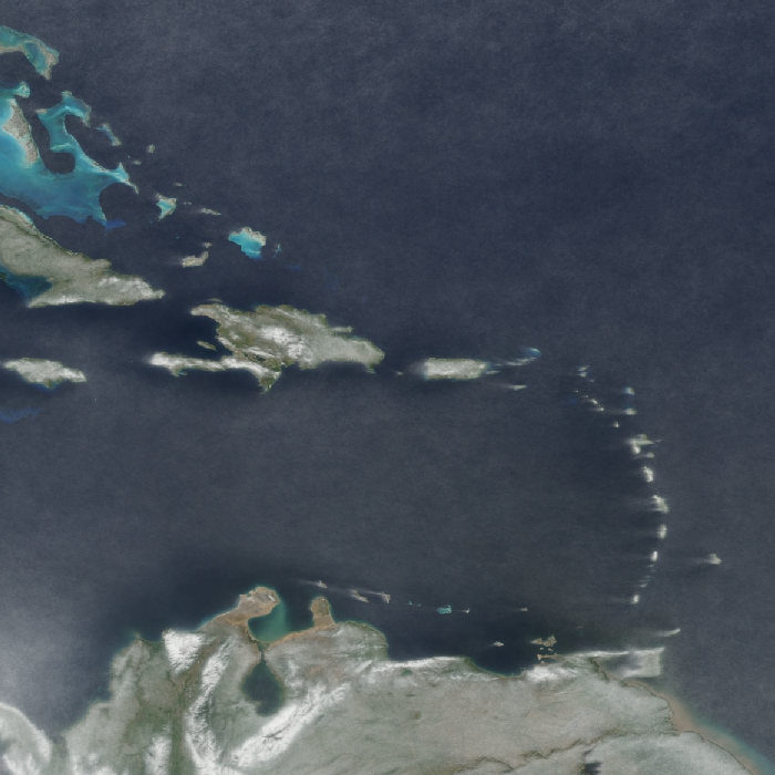
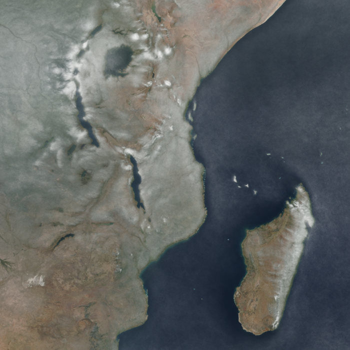
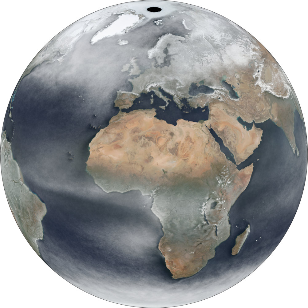
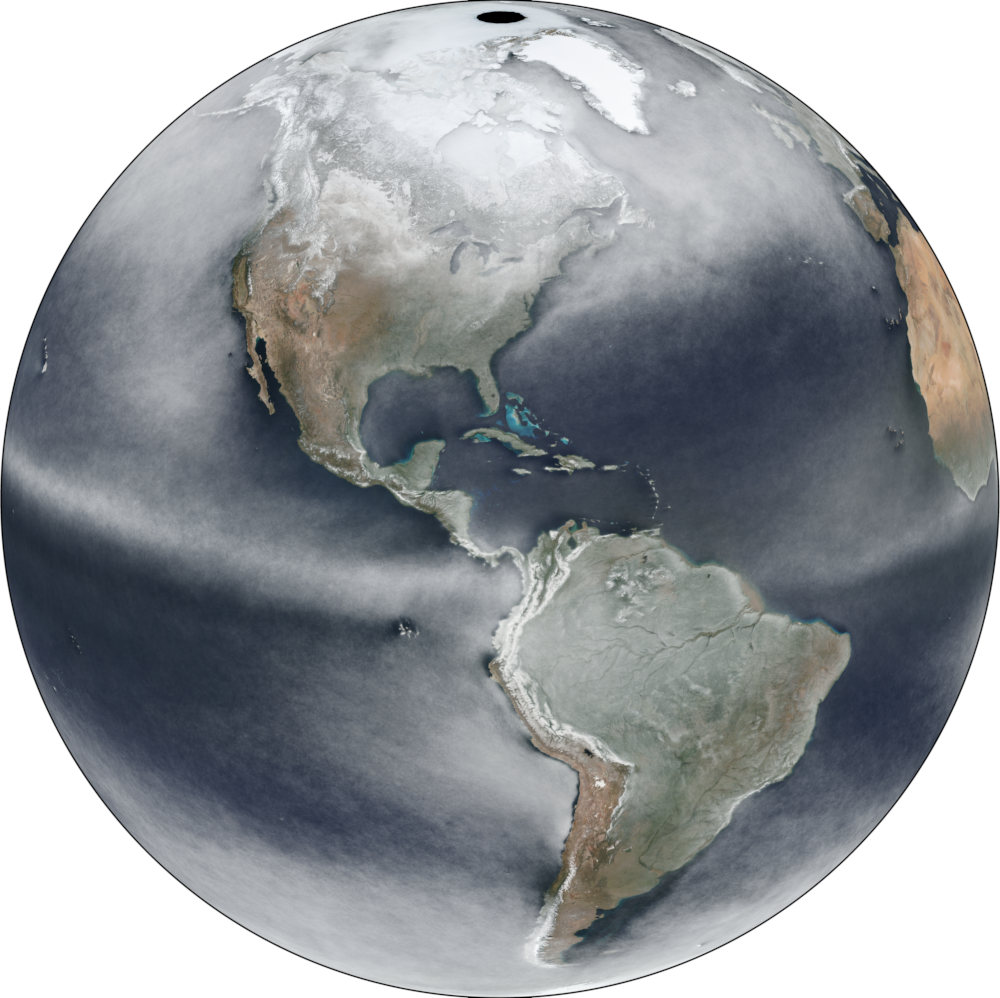
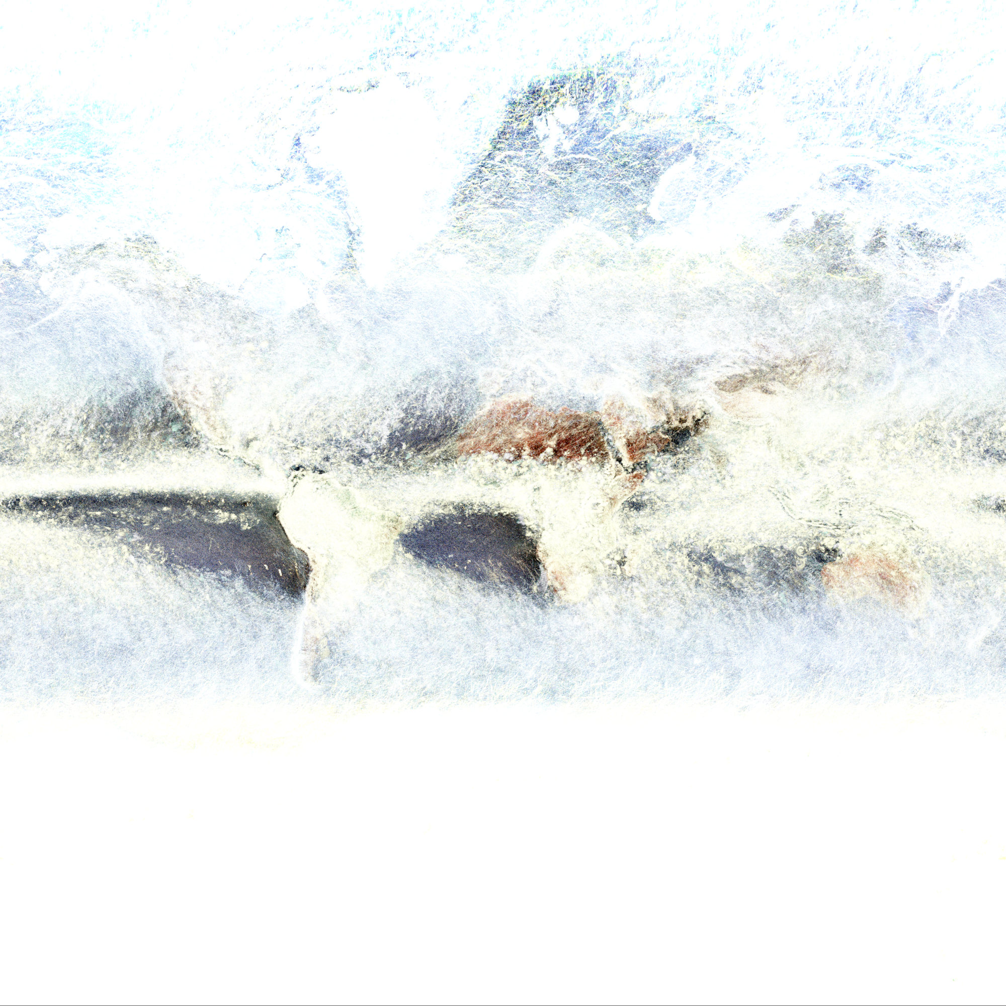
It’s also fun to look at the maximum to see cloudless regions (this image is highly exaggerated and does not make too much sense anyways):
Many thanks to Joshua Stevens for motivation and infos on data availability! The initial idea was of course inspired by Charlie ‘vruba’ Lyod‘s Cloudless atlas works. I explored imagery on https://worldview.earthdata.nasa.gov/, grabbed Soumi VIIRS images via https://wiki.earthdata.nasa.gov/display/GIBS/GIBS+API+for+Developers and processed it in GDAL. Poke me repeatedly to blog about the process please. (2022: Or don’t, I didn’t document it back then and can’t remember the final specifics. I think I did use imagemagick’s -evaluate-sequence median but might have done something in vips2 instead. The 2020 approach via GDAL is much easier.)
Full resolution, georeferenced imagery as Cloud-Optimized GeoTIFF:
*I said average but of course it is the median. The average or mean does not make much sense to use nor does it look any good. ;-)
Data-defined images in QGIS Atlas
Say you want to display a feature specific image on each page of a QGIS Atlas.
In my example I have a layer with two features:
{
  "type": "FeatureCollection",
  "features": [
    {
      "type": "Feature",
      "properties": {
        "image_path": "/tmp/1.jpeg"
      },
      "geometry": {
        "type": "Polygon",
        "coordinates": [[[9,53],[11,53],[11,54],[9,54],[9,53]]]
      }
    },
    {
      "type": "Feature",
      "properties": {
        "image_path": "/tmp/2.jpeg"
      },
      "geometry": {
        "type": "Polygon",
        "coordinates": [[[13,52],[14,52],[14,53],[13,53],[13,52]]]
      }
    }
  ]
}
And I also have two JPEG images, named “1.jpeg” and “2.jpeg” are in my /tmp/ directory, just as the “image_path” attribute values suggest.
The goal is to have a map for each feature and its image displayed on the same page.
Create a new print layout, enable Atlas, add a map (controlled by Atlas, using the layer) and also an image.
For the “image source” enable the data-defined override and use attribute(@atlas_feature, 'image_path') as expression.
That’s it, now QGIS will try to load the image referenced in the feature’s “image_path” value as source for the image on the Atlas page. Yay kittens!

