I like doing silly things in QGIS.
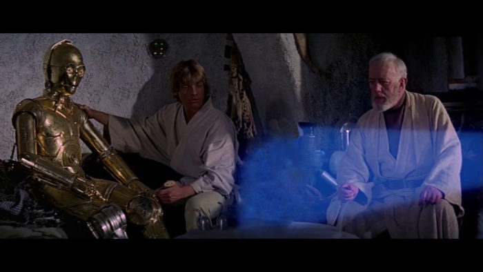
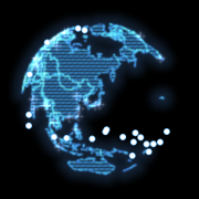
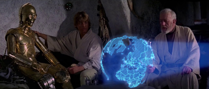
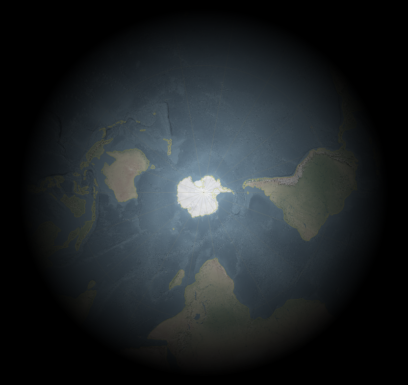
So I wanted to make a Star Wars hologram (you know, that “You’re my only hope” Leia one) showing real geodata. What better excuse for abusing QGIS’ Inverted Polygons and Raster Fills. So, here is what I did:
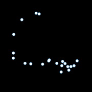
- Find some star wars hologram leia image.

- Crudly remove the princess (GIMP’s Clone and Healing tools work nicely for this).
- In QGIS create an empty Polygon-geometry Scratchpad layer and set the renderer to Inverted Polygons to fill the whole canvas.
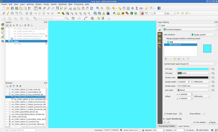
- Set the Fill to a Raster image Fill and load your image.
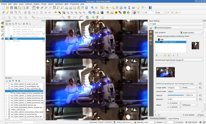
- Load some geodata, style it accordingly and rejoice.
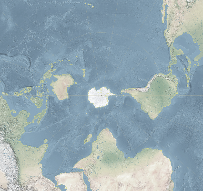
- Get some geodata. I used Natural Earth’s countries, populated places and tiny countries (to have some stuff in the oceans), all in 110m.
- Select a nice projection, I used “+proj=ortho +lat_0=39 +lon_0=139 +x_0=0 +y_0=0 +a=6371000 +b=6371000 +units=m +no_defs”.
- I used a three layer style for the countries:
- A Simple Line outline with color #4490f3, stroke width 0.3mm and the Dash Dot Line stroke style.
- A Line Pattern Fill with a spacing of 0.8mm, color #46a8f3 and a stroke width of 0.4mm.
- And on top of those, for some noisiness a black Line Pattern Fill rotated 45° with a spacing of 1mm and stroke width 0.1mm.
- Then the Feature Blending Mode Dodge to the Layer Rendering and aha!
- More special effects come from Draw Effects, I disabled Source and instead used a Blur (Gaussian, strength 2) to lose the crispness and also an Outer Glow (color #5da6ff, spread 3mm, blur radius 3) to, well, make it glow.


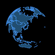


- I used a three layer style for the populated places:
- I used a Simple Marker using the “cross” symbol and a size of 1.8mm. The Dash Line stroke style gives a nice depth effect when in Draw Effects the Source is replaced with a Drop Shadow (1 Pixel, Blur radius 2, color #d6daff).
- A Blending Mode of Addition for the layer itself makes it blend nicely into the globe.
- I used a three layer style for the tiny countries:
- I used a white Simple Marker with a size of 1.2mm and a stroke color #79c7ff, stroke width 0.4mm.
- Feature Blending Mode Lighten makes sure that touching symbols blob nicely into each other.


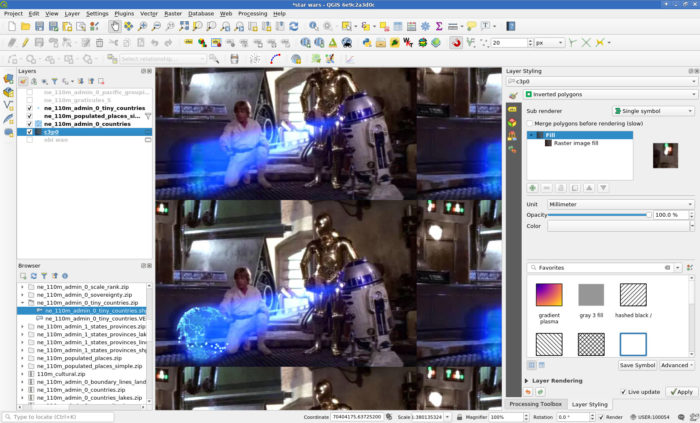
- You can now export the image at your screen resolution (I guess) using Project -> Import/Export or just make a screenshot.

- Or add some more magic with random offsets and stroke widths in combination with refreshing the layers automatically at different intervals:


 Hillshading
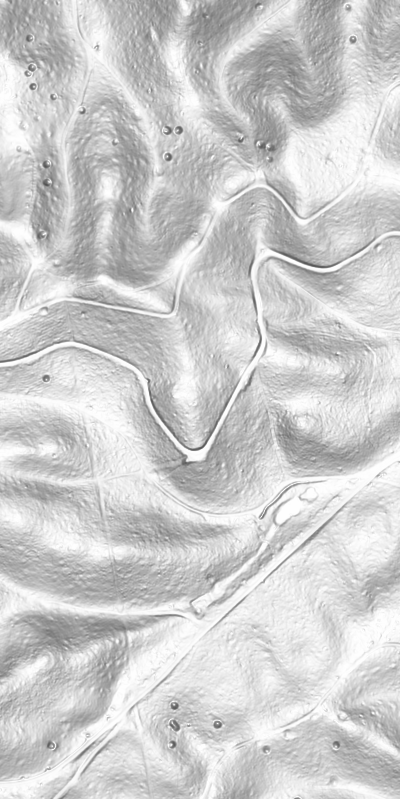 Overhead Hillshading
 Hillshading blended with Overhead Hillshading (Darken mode)
 Multidirectional Hillshading


